The MOS explorers, old and new

Two interactive widgets side by side: vizs.MOS_interactive as it was before this work, now frozen in biotuner.mos.legacy because the function in the repo delegates to the replacement — and biotuner.mos.mos_explorer.

Run this top to bottom in Jupyter. ipywidgets needs a live kernel; the widgets will not appear in a static render of this notebook.

Requirements: pip install ipywidgets plotly

import warnings
warnings.filterwarnings("ignore")

%matplotlib inline
import math
import matplotlib.pyplot as plt
import numpy as np

import biotuner.mos as M

plt.rcParams["figure.dpi"] = 96
print("ready")

C:\Users\skite\Documents\Github\biotuner\.claude\worktrees\epic-morse-ded0d5\biotuner\biotuner_object.py:11: DeprecationWarning: 
The `fooof` package is being deprecated and replaced by the `specparam` (spectral parameterization) package.
This version of `fooof` (1.1) is fully functional, but will not be further updated.
New projects are recommended to update to using `specparam` (see Changelog for details).
  from fooof import FOOOF

ready

1. The original — vizs.MOS_interactive, now mos.legacy.MOS_interactive

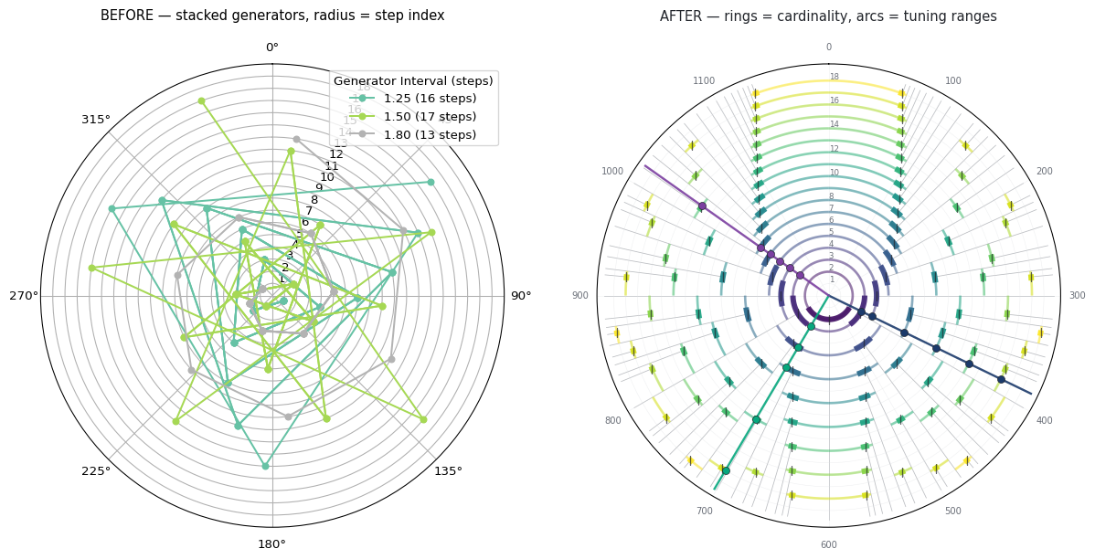
Five generator sliders (1.0–2.0) with toggles, a max-steps slider and a Play button. For each active generator it plots the stacked degrees as a spiral, radius = step index. It also tries to draw a dashed radial wherever two generators produce a coinciding tone.

It lives in biotuner.mos.legacy now — frozen, same maths, same defaults — because vizs.MOS_interactive delegates to the replacement and would otherwise leave the original reachable only through git show.

Two things to notice while using it. There are no rings, arcs, spokes or landmarks, so none of the paper’s readings are available; and the radius is the index of the stacked generator, not the cardinality of anything.

A third thing you will not notice: the dashed common-tone radials never appear. The test is exact float equality between independently computed angles, so it fires for no generator pair at all — measured, not assumed. That is why theory.common_tones uses a cents tolerance.

M.legacy.MOS_interactive()

The two figures, side by side

No widgets, just the output each one draws for the same three generators.

GENS = [1.25, 1.5, 1.8]

fig = plt.figure(figsize=(15, 7))
a1 = fig.add_subplot(1, 2, 1, projection="polar")
M.legacy.plot_MOS_spiral(GENS, max_steps=18, ax=a1)
a1.set_title("BEFORE — stacked generators, radius = step index", fontsize=11, pad=18)

a2 = fig.add_subplot(1, 2, 2, projection="polar")
M.plot_labyrinth(18, ax=a2, highlight=[M.generator_fraction(g) for g in GENS])
a2.get_legend().remove()
a2.set_title("AFTER — rings = cardinality, arcs = tuning ranges", fontsize=11, pad=18)
plt.show()

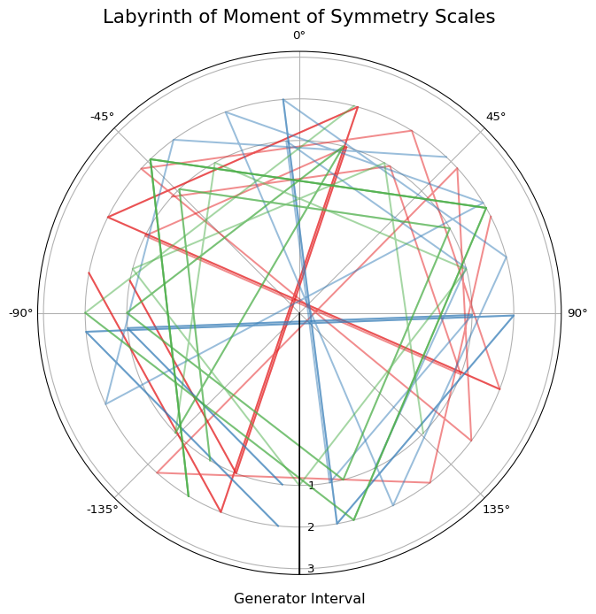
# And the old static one, for completeness. Every scale lands on radius 1 or 2.
M.legacy.plot_labyrinth([4 / 3, 3 / 2, 9 / 5], max_steps=16)

(<Figure size 768x768 with 1 Axes>,
 <PolarAxes: title={'center': 'Labyrinth of Moment of Symmetry Scales'}, xlabel='Generator Interval'>)

2. The replacement — mos_explorer

Same two good ideas — several generators at once, and their common tones — on top of the actual labyrinth. Drag a generator and the family recomputes, the wheel redraws, the summary updates and the fit against your signal is re-scored.

Controls:

gen 1…5	toggle a generator on or off; the first active one is focused
slider beside each	that generator, in cents
period ratio	the pseudo-octave — the paper treats it as a free parameter
max rings	outermost cardinality
cardinality	which ring of the focused generator’s family to inspect
overlays	signal peaks, named temperaments, coherence bands, common tones
common tol ¢	how close two generators’ tones must be to count as shared
▶ play scale	sonify the focused scale (needs pygame)
copy .scl	print a Scala file for it

# A synthetic stack of fifths, as used throughout the report.
PEAKS = [1.0, 1.125, 1.3333, 1.5, 1.6875]

M.mos_explorer(ratios=PEAKS)

Switch on gen 2 and drag it. With two generators active the dotted radial lines appear at their shared tones, and the text panel lists them. Two generators of the same equal division share all of it; a generator and its complement share only the root, because they build the same scale mirrored rather than the same set of pitches.

# Start with two generators already on: the fifth and the 31-EDO meantone fifth.
M.mos_explorer(ratios=PEAKS, generators=[3 / 2, 2 ** (18 / 31)], n_generators=3)

Bound to a real signal

Give it a compute_biotuner instead of raw ratios and the peaks come from the signal, weighted by amplitude, with the first generator seeded at the best-fitting one.

from biotuner.biotuner_object import compute_biotuner

rng = np.random.default_rng(7)
sf = 1000.0
t = np.arange(0, 30, 1 / sf)
base = 5.0
partials = [base, base * 1.5, base * 2.25, base * 3.375, base * 2.0]
amps = [1.0, 0.9, 0.75, 0.5, 0.65]
signal = sum(a * np.sin(2 * np.pi * f * t) for a, f in zip(amps, partials))
signal = signal + 0.25 * rng.standard_normal(t.size)

bt = compute_biotuner(sf, peaks_function="FOOOF", precision=0.1)
bt.peaks_extraction(signal, min_freq=2, max_freq=40, n_peaks=5)
print("peaks:", np.round(bt.peaks, 3))

M.mos_explorer(bt)

peaks: [ 5.    7.5   9.99 11.25 16.88]

3. fit_explorer — inspect the runners-up

The ranked fits, one per dropdown entry, each with its residuals and its position in the labyrinth. A close second is common, and the ranking is only as good as its parsimony penalty, so it is worth looking rather than trusting.

M.fit_explorer(bt.peaks_ratios, max_cardinality=16)

4. scratch_explorer — Fourier Scratching

A slider per Fourier coefficient. Moving one reshapes the whole play state at once, which is the point of the technique. It opens on the first partial, which strikes every tone exactly once in ascending order.

d12 = M.MOSScale.from_signature(5, 2, tuning=12)
M.scratch_explorer(M.christoffel_mode(d12))

5. labyrinth_plotly — no kernel needed

Hover-rich and zoomable, and with generator_slider=True it gets a precomputed slider, so the exported file stays interactive with nothing running behind it.

fig = M.labyrinth_plotly(16, peaks=bt.peaks_ratios, temperaments=True,
                         generator_slider=True, slider_steps=97)
fig

fig.write_html("labyrinth.html")
print("wrote labyrinth.html — opens in any browser, no Python required")

wrote labyrinth.html — opens in any browser, no Python required

6. The other labyrinths

Not interactive, but worth a look from here since everything is loaded.

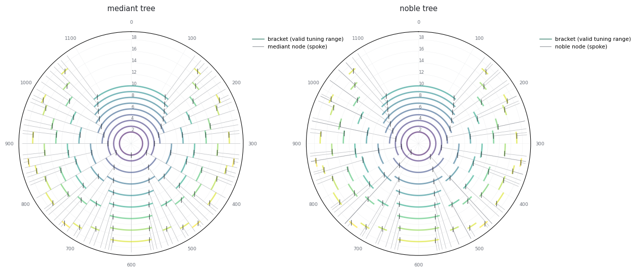
fig, axes = plt.subplots(1, 2, figsize=(14, 6), subplot_kw={"projection": "polar"})
M.plot_labyrinth_variant(rule=M.MEDIANT, max_cardinality=18, ax=axes[0])
M.plot_labyrinth_variant(rule=M.NOBLE, max_cardinality=18, ax=axes[1])
axes[0].set_title("mediant tree", fontsize=11, pad=14)
axes[1].set_title("noble tree", fontsize=11, pad=14)
plt.show()

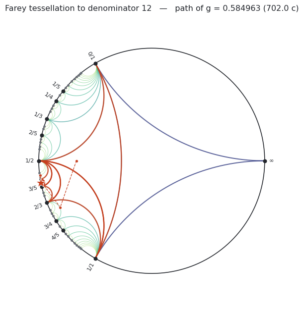
M.plot_farey_tessellation(12, highlight_generator=math.log2(3 / 2))
plt.show()

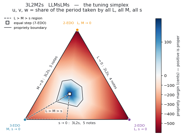
M.plot_ternary_simplex("LLMsLMs", field="propriety")
plt.show()

7. web_explorer — the scale as a figure

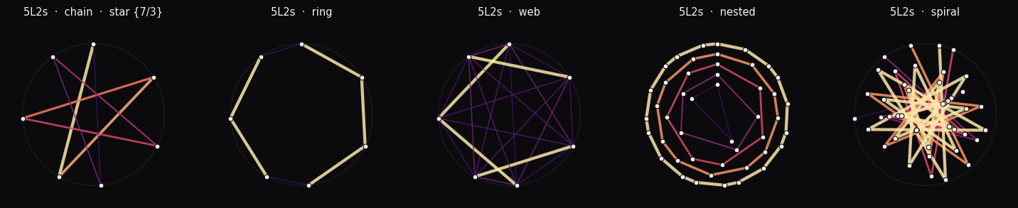
The design counterpart. Drag the generator and the star polygon reforms; step through the modes and the silhouette rotates; switch style and the same scale is redrawn five ways.

Each style encodes something rather than decorating:

style	what the shape means
chain	degrees joined in generator order — a star polygon {N/d}, the circle of fifths made visible
ring	degrees joined in pitch order — edge lengths are the step sizes
web	every interval, weighted by harmonicity — the bright heavy lines are the consonances
nested	the whole family, so the embedding shows as concentric shapes
spiral	the original stacked-generator figure, rebuilt

The star’s density is the modular inverse of Carey’s WF number, not the number itself. For the diatonic, WF(7, 2) means one scale step is two fifths, so one fifth is four scale steps and the figure is the heptagram {7/3}.

M.web_explorer(3 / 2)

# All five styles for one scale.
d31 = M.MOSScale.from_signature(5, 2, tuning=31)
fig, axes = plt.subplots(1, 5, figsize=(19, 4.2))
for ax, st in zip(axes, M.STYLES):
    M.plot_scale_web(d31, st, ax=ax, palette="noir", max_cardinality=29)
plt.show()

# The seven diatonic modes as silhouettes — one boundary moves per step.
fig, axes = plt.subplots(1, 7, figsize=(21, 3.6))
for i, ax in enumerate(axes):
    M.plot_scale_web(d31, "ring", mode=i, ax=ax, palette="ink", title=d31.mode(i).name)
plt.show()

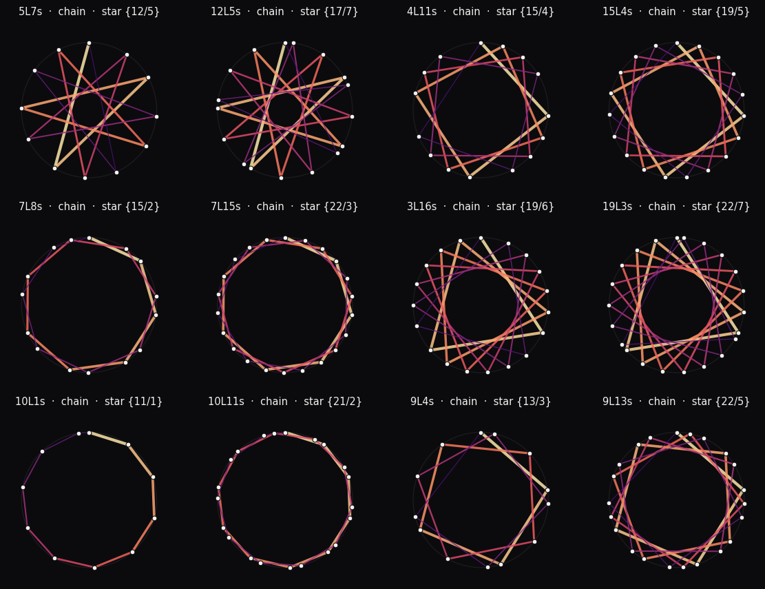
# A design sheet: two scales from each of several generators.
scales = []
for g in [3/2, 2**(316/1200), 2**(163.9/1200), 2**(380/1200), 2**(117/1200), 2**(271/1200)]:
    scales += [s for s in M.mos_family(g, 24) if 5 <= s.cardinality <= 24][-2:]
M.plot_web_gallery(scales[:12], "chain", palette="noir", n_cols=4, panel=3.0)
plt.show()

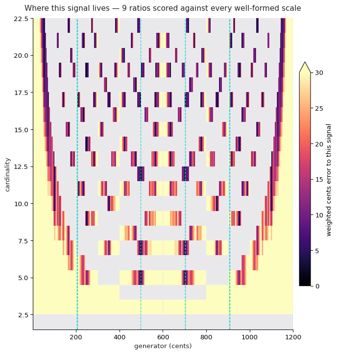
8. fit_field — where the signal lives, everywhere at once

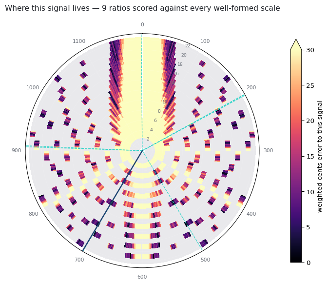
fit_mos returns a ranked shortlist, which hides how the winner sits among its neighbours. This scores the whole labyrinth against the same ratios.

The finding it exists to show: a signal is usually compatible with several disconnected regions, not one. islands() counts them, treating the generator axis as circular because the labyrinth is.

Note the field samples the generator axis and does not refine, so its best cell will not match fit_mos to the last cent — and it applies no parsimony penalty, so it will usually name a larger scale. Both differences are the two functions doing their different jobs.

field = M.fit_field(bt.peaks_ratios, max_cardinality=22, resolution=760)
print(f"coverage       {field.coverage:.1%} of cells hold a well-formed scale at all")
print(f"best cell      {field.best()}")
print(f"islands @3 c   {field.islands(3.0)}")
print(f"islands @1 c   {field.islands(1.0)}")
print(f"chance @12     {field.chance_error(12):.2f} c")

coverage       36.5% of cells hold a well-formed scale at all
best cell      {'cardinality': 12, 'generator': 0.4144736842105263, 'generator_cents': 497.3684210526316, 'error_cents': 0.8153531518111823}
islands @3 c   68
islands @1 c   18
chance @12     25.00 c

# The shortlist's winner, to mark on the field.
fit = M.fit_mos(bt.peaks_ratios, max_cardinality=22)[0]
print("marking", fit.signature, f"at {fit.error_cents:.2f} c")

M.plot_fit_field(field, mark=fit.scale)
plt.show()

marking 2L3s at 0.58 c

# Cartesian is easier to read values off.
M.plot_fit_field(field, polar=False)
plt.show()

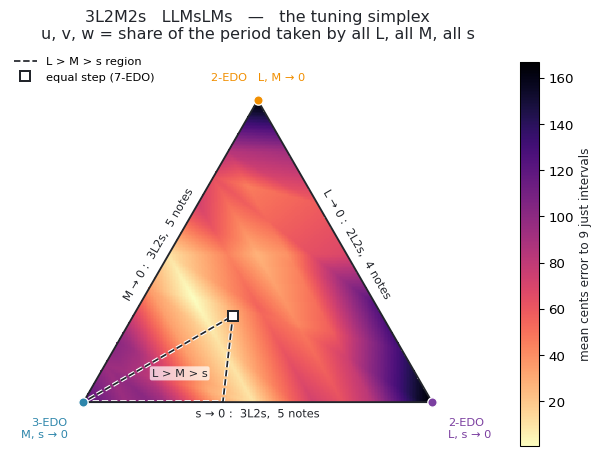
The same idea works on the ternary simplex without any new code: the just-intonation field already takes a target set, so passing your own ratios turns it into a fit field over a three-step-size scale’s tuning space.

M.plot_ternary_simplex("LLMsLMs", field="ji_error", targets=bt.peaks_ratios)
plt.show()

9. The last four explorers

simplex_explorer — the ternary tuning space

A three-step-size scale’s tuning space is a triangle, so this is mos_explorer’s counterpart for it. Two sliders place u and v; w = 1 - u - v follows, clamped so the point never leaves the open simplex (a zero step is not a ternary scale).

M.simplex_explorer("LLMsLMs")

trajectory_explorer — scrub a recording

Step through the windows of a mos_trajectory, watching the fit move around the labyrinth with the path so far drawn behind it. Windows where nothing could be fitted are shown as such rather than skipped.

# A recording that changes its mind half way through: fifteen seconds built on a
# chain of fifths, then fifteen on a chain of major thirds. A single fit over the
# whole thing would average the two into a scale that is in neither half.
def _chain(ratio, n=5):
    return [base * ratio ** k for k in range(n)]

half = t.size // 2
switching = np.concatenate([
    sum(a * np.sin(2 * np.pi * f * t[:half]) for a, f in zip(amps, _chain(1.5))),
    sum(a * np.sin(2 * np.pi * f * t[half:]) for a, f in zip(amps, _chain(1.25))),
])
switching = switching + 0.25 * rng.standard_normal(switching.size)

traj = M.mos_trajectory(switching, sf, window_sec=6.0, step_sec=3.0,
                        peaks_function="FOOOF", precision=0.1, n_peaks=5,
                        max_cardinality=16)
M.trajectory_explorer(traj)

C:\Users\skite\AppData\Local\Programs\Python\Python310\lib\site-packages\scipy\signal\_spectral_py.py:790: UserWarning: nperseg = 10000 is greater than input length  = 6000, using nperseg = 6000
  freqs, _, Pxy = _spectral_helper(x, y, fs, window, nperseg, noverlap,

C:\Users\skite\AppData\Local\Programs\Python\Python310\lib\site-packages\scipy\signal\_spectral_py.py:790: UserWarning: nperseg = 10000 is greater than input length  = 6000, using nperseg = 6000
  freqs, _, Pxy = _spectral_helper(x, y, fs, window, nperseg, noverlap,

C:\Users\skite\AppData\Local\Programs\Python\Python310\lib\site-packages\scipy\signal\_spectral_py.py:790: UserWarning: nperseg = 10000 is greater than input length  = 6000, using nperseg = 6000
  freqs, _, Pxy = _spectral_helper(x, y, fs, window, nperseg, noverlap,

C:\Users\skite\AppData\Local\Programs\Python\Python310\lib\site-packages\scipy\signal\_spectral_py.py:790: UserWarning: nperseg = 10000 is greater than input length  = 6000, using nperseg = 6000
  freqs, _, Pxy = _spectral_helper(x, y, fs, window, nperseg, noverlap,

C:\Users\skite\AppData\Local\Programs\Python\Python310\lib\site-packages\scipy\signal\_spectral_py.py:790: UserWarning: nperseg = 10000 is greater than input length  = 6000, using nperseg = 6000
  freqs, _, Pxy = _spectral_helper(x, y, fs, window, nperseg, noverlap,

C:\Users\skite\AppData\Local\Programs\Python\Python310\lib\site-packages\scipy\signal\_spectral_py.py:790: UserWarning: nperseg = 10000 is greater than input length  = 6000, using nperseg = 6000
  freqs, _, Pxy = _spectral_helper(x, y, fs, window, nperseg, noverlap,

C:\Users\skite\AppData\Local\Programs\Python\Python310\lib\site-packages\scipy\signal\_spectral_py.py:790: UserWarning: nperseg = 10000 is greater than input length  = 6000, using nperseg = 6000
  freqs, _, Pxy = _spectral_helper(x, y, fs, window, nperseg, noverlap,

C:\Users\skite\AppData\Local\Programs\Python\Python310\lib\site-packages\scipy\signal\_spectral_py.py:790: UserWarning: nperseg = 10000 is greater than input length  = 6000, using nperseg = 6000
  freqs, _, Pxy = _spectral_helper(x, y, fs, window, nperseg, noverlap,

C:\Users\skite\AppData\Local\Programs\Python\Python310\lib\site-packages\scipy\signal\_spectral_py.py:790: UserWarning: nperseg = 10000 is greater than input length  = 6000, using nperseg = 6000
  freqs, _, Pxy = _spectral_helper(x, y, fs, window, nperseg, noverlap,

dissonance_explorer — where Dynamic Tonality earns its keep

Top: sensory roughness against interval width, harmonic timbre versus matched, with the scale’s own degrees marked. Watch the matched curve’s minima pull onto the degrees.

Bottom: total scale dissonance as the generator sweeps its whole valid range, with the coherent band shaded. This is the panel that shows where matching wins and where it does not.

M.dissonance_explorer(5, 2, n_partials=8)

Two things worth knowing before you read the numbers.

At the partials slider’s floor the two timbres are identical. A matched spectrum cannot move partial 1, and with an octave period it cannot move partial 2 either, so at n_partials=2 the matched ratios are exactly [1.0, 2.0] and neither timbre is smoother. The explorer says so rather than reporting a phantom result.

Matching helps more inside the coherent range, not outside. Measured over 241 generators at 8 partials:

scale	inside coherent	outside
5L2s	wins 88.0 %, median +3.39 %	wins 75.9 %, median +2.64 %
4L3s	wins 84.1 %, median +2.09 %	wins 83.0 %, median +1.81 %
7L5s	wins 95.5 %, median +2.10 %	wins 91.5 %, median +1.98 %
2L5s	wins 75.9 %, median +1.53 %	wins 69.5 %, median +0.45 %

The exact win fractions shift a little with the sampling grid; the direction does not.

matrix_explorer — watch propriety break

Left: the interval matrix, rows = starting degree, columns = generic class. Right: the specific sizes each generic class takes. When two adjacent classes’ bands overlap, some third is wider than some fourth — that overlap is impropriety, and it appears exactly as Blackwood’s R crosses 2.

M.matrix_explorer(5, 2)

10. Morphing — the labyrinth as a map you travel

Everything above reads the labyrinth as a place: rings, arcs, landmarks, a point where your signal sits. mos.morph reads it as a map and asks the next question — how do you get from this scale to that one?

There are three honest answers and they disagree.

strategy	what is held	what moves	stays well-formed?
tuning	the structure nL, ns	the generator, continuously	yes — it slides along one arc
tree	nothing but well-formedness	the signature, one legal hop at a time	yes — it jumps between rings
voice	the note count	every tone, straight to its partner	no — almost every frame is off the map

They are different journeys between the same two places, not three spellings of one, and the arithmetic says so: between one pair of scales below their totals differ by a factor of nineteen.

tuning_morph — hold the structure, slide the generator

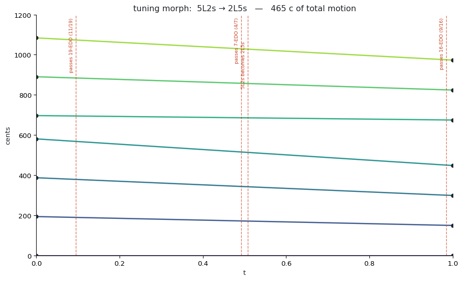
This is the Dynamic Tonality knob. Seven notes stay seven notes and the two step sizes co-vary; nothing about the scale’s identity changes except its tuning. Except once. Where the generator passes an equalized landmark the large step and the small step trade places, and the scale meets its own inverse coming the other way.

Meantone to anti-meantone is that trip. 5L2s at 31-EDO has a 696.8 ¢ fifth, its inverse 2L5s a 674.7 ¢ one, and 7-EDO’s 685.7 ¢ sits between them. In the summary the crossing at t≈0.49 and the flip at t≈0.51 are one event reported twice — from outside as a tuning the scale passes through, from inside as a change of signature. In the trajectory it is the instant the seven lines are evenly spaced: before it the whole tones are the wide steps, after it they are the narrow ones, and at the crossing there is no difference left to have.

d31 = M.MOSScale.from_signature(5, 2, tuning=31)
slide = M.tuning_morph(d31, d31.inverse, steps=64)
print(slide.summary())

M.plot_morph_trajectory(slide)
plt.show()

tuning morph:  5L2s (696.8 c) -> 2L5s (674.7 c)
  frames         64
  route          5L2s -> 2L5s
  voice motion   464.5 c total
  every frame is a well-formed scale
    t=0.095  passes 19-EDO (11/19)
    t=0.492  passes 7-EDO (4/7)
    t=0.508  5L2s becomes 2L5s: the large and small steps trade places
    t=0.984  passes 16-EDO (9/16)

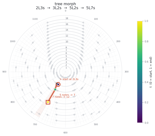
tree_morph — change the structure, one legal move at a time

A tuning morph cannot add a note: holding the structure fixed is precisely refusing to. Changing the note count means hopping rings, and the labyrinth has its own connectivity for that. A signature’s two children are the Stern–Brocot mediants (nL, nL+ns) and (nL+ns, ns) — which is why 5L2s’s child 5L7s has exactly the twelve notes embedding predicts — its parent is the subtractive Euclidean step back up, and one further move swaps (nL, ns) for (ns, nL) across the landmark they share.

Pentatonic to chromatic is a walk up this tree. Shortest routes are rarely unique, so the tie-break carries the musical judgement: among equally short routes, take the one that stays small longest and adds notes only when it must. Both routes printed below are three hops and every hop in both is legal; the taken one reaches twelve notes at the end, the rejected one reaches twelve a step early and then sits there.

from biotuner.mos.morph import signature_children, signature_parent, signature_route

print("children of 5L2s ", signature_children(5, 2))
print("parent of 5L2s   ", signature_parent(5, 2))
print()

taken = signature_route((2, 3), (5, 7))
detour = [(2, 3), (2, 5), (7, 5), (5, 7)]
for name, r in (("taken   ", taken), ("rejected", detour)):
    print(name, " -> ".join(f"{a}L{b}s" for a, b in r),
          "  notes:", [a + b for a, b in r])
print()

penta = M.MOSScale.from_signature(2, 3, tuning=12)
chroma = M.MOSScale.from_signature(5, 7, tuning=12)
climb = M.tree_morph(penta, chroma)
print(climb.summary())

M.plot_morph_path(climb)
plt.show()

children of 5L2s  [(5, 7), (7, 2)]
parent of 5L2s    (3, 2)

taken    2L3s -> 3L2s -> 5L2s -> 5L7s   notes: [5, 5, 7, 12]
rejected 2L3s -> 2L5s -> 7L5s -> 5L7s   notes: [5, 7, 12, 12]

tree morph:  2L3s (700.0 c) -> 5L7s (700.0 c)
  frames         4
  route          2L3s -> 3L2s -> 5L2s -> 5L7s
  voice motion   2500.0 c total
  every frame is a well-formed scale
    t=0.000  start at 2L3s
    t=0.667  5 notes -> 7: 5L2s
    t=1.000  7 notes -> 12: 5L7s

voice_morph — move the notes and let the structure go

The third strategy asks what you would actually hear. Each tone glides the shorter way round the circle to its counterpart, and where the two scales have different note counts tones split or merge — the same thing that happens at a landmark when a step size shrinks to nothing. Nothing holds the frames in between to being scales, and generally they are not: MorphStep.wellformedness is the number of cents each frame misses being one by, and the lower panel of the trajectory plot tracks it.

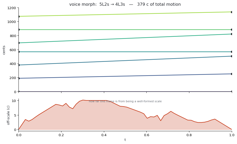
Here is the trade, priced. 5L2s and 4L3s in 19-EDO share three of their seven tones, so the voices barely have to move. The tuning morph between the same two scales is legal in every single frame and pays for it: to keep the structure intact it drags all seven tones through 3-EDO at t≈0.56, where they collapse onto three pitches, and back out. Nineteen times the motion, for the privilege of never leaving the map.

a19 = M.MOSScale.from_signature(5, 2, tuning=19)
b19 = M.MOSScale.from_signature(4, 3, tuning=19)
shared = sorted(set(np.round(a19.cents, 1)) & set(np.round(b19.cents, 1)))
print("shared tones:", ", ".join(f"{c:.1f} c" for c in shared))
print()

glide = M.voice_morph(a19, b19, steps=64)
slide2 = M.tuning_morph(a19, b19, steps=64)
print(glide.summary())
print()
print(slide2.summary())
print()
print(f"voice {glide.voice_leading_distance():.0f} c  vs  "
      f"tuning {slide2.voice_leading_distance():.0f} c  "
      f"({slide2.voice_leading_distance() / glide.voice_leading_distance():.0f}x)")

M.plot_morph_trajectory(glide)
plt.show()

shared tones: 0.0 c, 568.4 c, 884.2 c

voice morph:  5L2s (694.7 c) -> 4L3s (884.2 c)
  frames         64
  route          5L2s -> (off-scale) -> 4L3s
  voice motion   378.9 c total
  leaves the labyrinth for 62 of 64 frames, by up to 10.2 c

tuning morph:  5L2s (694.7 c) -> 4L3s (884.2 c)
  frames         64
  route          5L2s -> 3L4s -> 4L3s
  voice motion   7332.3 c total
  every frame is a well-formed scale
    t=0.032  passes 12-EDO (7/12)
    t=0.127  passes 5-EDO (3/5)
    t=0.238  passes 13-EDO (8/13)
    t=0.286  passes 8-EDO (5/8)
    t=0.556  passes 3-EDO (2/3)
    t=0.571  5L2s becomes 3L4s: the large and small steps trade places
    t=0.857  passes 7-EDO (5/7)
    t=0.873  3L4s becomes 4L3s: the large and small steps trade places

voice 379 c  vs  tuning 7332 c  (19x)

All three at once

Read down a column for one journey, across a row to compare them. Top: the path on the labyrinth, where the shape alone says which strategy it was — a slide along one arc, a climb between rings, and one that is mostly absent, its two banks joined by a dotted line across the frames it spends off the map. Bottom: the same three journeys as voice leading, with their totals.

fig, morphs = M.plot_morph_comparison(a19, b19, steps=64)
plt.show()

for name, mm in morphs.items():
    off = sum(1 for s in mm if not s.is_well_formed)
    print(f"{name:7s} {len(mm):3d} frames  {mm.voice_leading_distance():7.0f} c  "
          f"{off:3d} off-scale   {' -> '.join(mm.signatures())}")

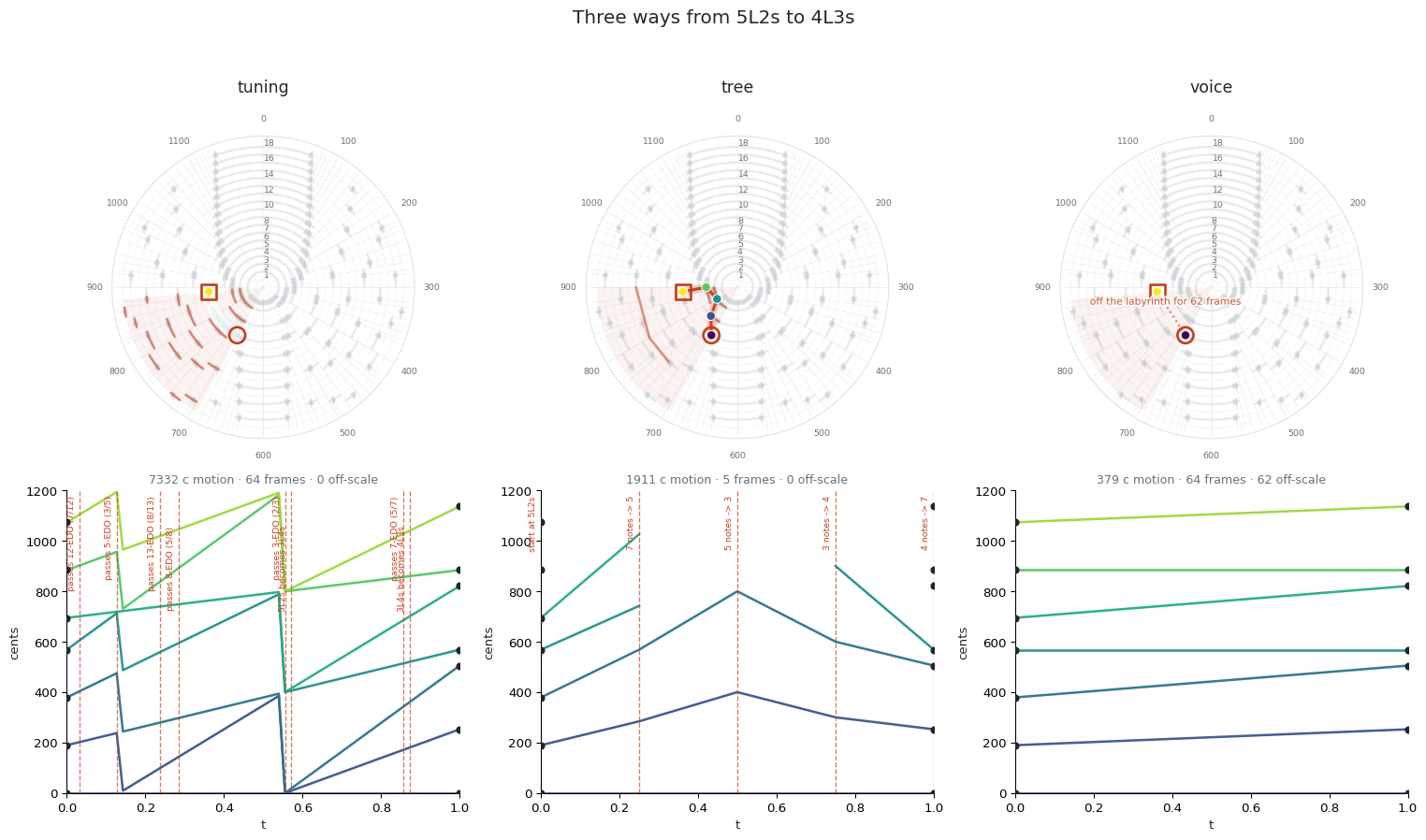
tuning   64 frames     7332 c    0 off-scale   5L2s -> 3L4s -> 4L3s
tree      5 frames     1911 c    0 off-scale   5L2s -> 3L2s -> 1L2s -> 1L3s -> 4L3s
voice    64 frames      379 c   62 off-scale   5L2s -> (off-scale) -> 4L3s

morph_explorer — drive it yourself

from L/from s and to L/to s set the two signatures, EDO tunes both endpoints, and strategy switches the journey with the pair held fixed — which is how you see why the three disagree rather than merely that they do. Move to s from 3 to 7 and the tree route lengthens from four hops to five while the voice morph is unchanged in shape, still start, off the map, end.

The same move takes tuning away entirely, and the widget lets you find that out by pressing the button rather than by hiding it: it prints that you cannot slide a seven-note scale into an eleven-note one. That is the lesson, not an error. (Two signatures with a common factor, and signatures the chosen EDO cannot spell — 5L7s has no 19-EDO generator — have no endpoint to build from at all; change EDO first.)

listen renders the current morph with morph_audio — every tone of the scale as one continuous glide, so what you hear is the movement rather than a sequence of chords — and drops an audio player below the plot; seconds sets its length. The nineteen-fold difference above is far more obvious in the ear than in the figure: one morph wanders through three equal divisions on its way, the other barely moves.

M.morph_explorer((5, 2), (4, 3), tuning=19)