Resonance & Connectivity Cookbook

A practical tour of biotuner.resonance, biotuner.harmonic_spectrum, and biotuner.harmonic_connectivity — the three modules that together cover single-signal harmonic analysis and cross-channel connectivity.

This notebook walks through ten workflow categories:

1. Setup — synthetic signals + strategy discovery

2. H-only spectrum — compute_harmonic_spectrum

3. Full single-signal R(f) — compute_resonance, and why surrogate normalization is needed for H ≠ PC ≠ R discrimination

4. Swapping kernels — harmonic kernel

5. Swapping coupling metrics — including the n:m convention rule, with a cross-channel example that visibly separates PLV from PLI/wPLI

6. Swapping ratio kernels — binary vs fraction, with a 10:17 mode-lock that only the fraction kernel can test

7. Swapping combine rules — with H and PC peaks at different bins

8. Surrogate-null normalization — with_surrogate_null

9. Cross-channel resonance — compute_cross_resonance, 3 reducer flavors

10. Connectivity matrices + statistical inference

The cells are self-contained — each section can be run independently after the “Setup” block has been executed.

1. Setup

Imports + small helpers + synthetic-signal generators.

import numpy as np
import matplotlib.pyplot as plt

# biotuner.resonance — single-signal H × PC = R machinery
from biotuner.resonance import (
    compute_resonance, ResonanceConfig, ResonanceResult,
    with_surrogate_null, list_strategies, results_to_dataframe,
)

# biotuner.harmonic_spectrum — narrow H-only entry point
from biotuner.harmonic_spectrum import compute_harmonic_spectrum

# biotuner.harmonic_connectivity — cross-channel APIs
from biotuner.harmonic_connectivity import (
    harmonic_connectivity, compute_cross_resonance, CrossResonanceResult,
)

%matplotlib inline
plt.rcParams.update({"figure.dpi": 110, "lines.linewidth": 1.4,
                      "axes.spines.top": False, "axes.spines.right": False})

SF = 500   # sampling frequency for all examples

def pink_noise(n, sf, seed=0):
    rng = np.random.default_rng(seed)
    w = rng.standard_normal(n)
    f = np.fft.rfftfreq(n, 1/sf); f[0] = f[1]
    return np.fft.irfft(np.fft.rfft(w) / np.sqrt(f), n=n)

def harmonic_signal(sf=SF, duration=8.0, freqs=(5, 10, 20, 40), amp_decay=0.7, seed=0):
    """Phase-locked harmonic stack of sinusoids on pink-noise background."""
    t = np.arange(int(sf * duration)) / sf
    sig = sum((amp_decay ** i) * np.sin(2 * np.pi * f * t) for i, f in enumerate(freqs))
    sig += 0.05 * pink_noise(len(t), sf, seed=seed)
    return sig

def alpha_burst_signal(sf=SF, duration=8.0, alpha_freq=10.0, n_bursts=6, seed=0):
    """EEG-like: 1/f background + Hann-windowed alpha bursts."""
    rng = np.random.default_rng(seed)
    n = int(sf * duration); t = np.arange(n) / sf
    sig = 1.0 * pink_noise(n, sf, seed=seed)
    burst_times = np.linspace(0.5, duration - 1.0, n_bursts) + rng.uniform(-0.1, 0.1, size=n_bursts)
    for bt in burst_times:
        idx = (t >= bt) & (t <= bt + 0.6)
        local = t[idx] - bt
        win = np.sin(np.pi * local / 0.6) ** 2
        sig[idx] += 2.0 * win * np.sin(2 * np.pi * alpha_freq * local + rng.uniform(0, 2 * np.pi))
    return sig

def detuned_pair_signal(sf=SF, duration=30.0, seed=0):
    """Two pairs that both LOOK like 1:2 harmonic stacks in the PSD, but
    only one is actually phase-locked:

      * 6 + 12 Hz — EXACT 1:2 ratio, phase-locked (high H, high PC, high R)
      * 9 + 18.5 Hz — slightly detuned (18.5/9 = 2.056 within binary's 5%
        tolerance, so H still sees it as 1:2) but the real phase relation
        drifts (low PC, low R)

    Pedagogical lesson: H reflects PSD shape; only the surrogate-z-scored
    R distinguishes real coupling from same-PSD impostors.
    """
    rng = np.random.default_rng(seed)
    n = int(sf * duration); t = np.arange(n) / sf
    phi = 2 * np.pi * 6 * t + 0.3
    locked = 1.2 * np.sin(phi) + 0.8 * np.sin(2 * phi + 0.4)
    detuned = (1.2 * np.sin(2 * np.pi * 9.0 * t + rng.uniform(0, 2 * np.pi))
               + 0.8 * np.sin(2 * np.pi * 18.5 * t + rng.uniform(0, 2 * np.pi)))
    lone = 0.7 * np.sin(2 * np.pi * 23 * t + 1.7)
    bg = 0.15 * pink_noise(n, sf, seed=seed + 99)
    return locked + detuned + lone + bg

def coupled_channels(sf=SF, duration=12.0, mode='lagged', seed=0):
    """Two channels coupled at 10 Hz under three coupling regimes:

      mode='zero_lag' : φ_A = φ_B exactly (volume-conduction artifact)
      mode='lagged'   : φ_B = φ_A + π/3 (genuine lagged coupling)
      mode='uncoupled': independent random phases (no coupling)

    Use this to compare phase-coupling metrics — PLV detects all three
    locked cases, PLI/wPLI suppress the zero-lag one.
    """
    rng = np.random.default_rng(seed)
    n = int(sf * duration); t = np.arange(n) / sf
    phi = 2 * np.pi * 10 * t
    sig_a = np.sin(phi) + 0.3 * pink_noise(n, sf, seed=seed + 1)
    if mode == 'zero_lag':
        sig_b = np.sin(phi) + 0.3 * pink_noise(n, sf, seed=seed + 2)
    elif mode == 'lagged':
        sig_b = np.sin(phi + np.pi / 3) + 0.3 * pink_noise(n, sf, seed=seed + 2)
    elif mode == 'uncoupled':
        # Random-walk phase: φ_B drifts independently — same PSD peak at 10 Hz,
        # but the phase relation to φ_A is destroyed over time.
        dphi = rng.standard_normal(n) * 1.0 * np.sqrt(1.0 / sf)
        sig_b = (np.sin(2 * np.pi * 10 * t + np.cumsum(dphi))
                 + 0.3 * pink_noise(n, sf, seed=seed + 2))
    else:
        raise ValueError(mode)
    return sig_a, sig_b

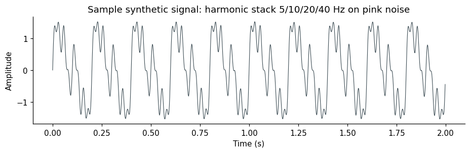
# Display a sample signal
sig = harmonic_signal()
fig, ax = plt.subplots(figsize=(10, 2.5))
t = np.arange(len(sig))/SF
ax.plot(t[:int(SF*2)], sig[:int(SF*2)], color='#37474f', lw=0.7)
ax.set_xlabel("Time (s)"); ax.set_ylabel("Amplitude")
ax.set_title("Sample synthetic signal: harmonic stack 5/10/20/40 Hz on pink noise")
plt.show()

1b. Discovery: what strategies are available?

list_strategies() prints every registered kernel, coupling metric, combine rule, etc. All names returned are valid for the corresponding ResonanceConfig field.

list_strategies()

HARMONIC_KERNELS (2)
  - harmsim
  - subharm_tension

RATIO_KERNELS (2)
  - binary
  - fraction

PHASE_ESTIMATORS (1)
  - stft

PAIRWISE_COUPLING_METRICS (6)
  - nm_pli  [phase]
  - nm_plv  [phase]
  - nm_plv_canonical  [phase]
  - nm_rrci  [phase]
  - nm_wpli  [phase]
  - nm_wpli_complex  [analytic]

HIGHER_ORDER_COUPLING_METHODS (0)
  (none — see plan §5 for the Phase 2/3 additions)

PERSISTENCE_METHODS (0)
  (none — see plan §5 for the Phase 2/3 additions)

COMBINE_RULES (5)
  - geomean
  - harmmean
  - min
  - product
  - weighted_log

SURROGATE_TYPES (0)
  (none — see plan §5 for the Phase 2/3 additions)

{'HARMONIC_KERNELS': {'harmsim': <function biotuner.resonance.kernels_harmonic.kernel_harmsim(freqs_i: numpy.ndarray, freqs_j: numpy.ndarray, *, diagonal: float = None, **_unused) -> numpy.ndarray>,
  'subharm_tension': <function biotuner.resonance.kernels_harmonic.kernel_subharm_tension(freqs_i: numpy.ndarray, freqs_j: numpy.ndarray, *, n_harms: int = 10, delta_lim: float = 20, min_notes: int = 2, diagonal: float = None, **_unused) -> numpy.ndarray>},
 'RATIO_KERNELS': {'binary': <function biotuner.resonance.kernels_ratio.binary_nm_kernel(freqs_i: numpy.ndarray, freqs_j: numpy.ndarray, *, max_nm: int = 3, tolerance: float = 0.05, fallback_to_1_1: bool = True, **_unused)>,
  'fraction': <function biotuner.resonance.kernels_ratio.fraction_kernel(freqs_i: numpy.ndarray, freqs_j: numpy.ndarray, *, max_denom: int = 16, beta: float = 1.0, **_unused)>},
 'PHASE_ESTIMATORS': {'stft': <function biotuner.resonance.phase_estimators.stft_phase(signal: numpy.ndarray, sf: float, *, precision_hz: float, noverlap: int = 10, smoothness: float = 1, **_unused) -> numpy.ndarray>},
 'PAIRWISE_COUPLING_METRICS': {'nm_plv': <function biotuner.resonance.coupling.nm_plv(phase_i: numpy.ndarray, phase_j: numpy.ndarray, n: int, m: int) -> float>,
  'nm_pli': <function biotuner.resonance.coupling.nm_pli(phase_i: numpy.ndarray, phase_j: numpy.ndarray, n: int, m: int) -> float>,
  'nm_wpli': <function biotuner.resonance.coupling.nm_wpli(phase_i: numpy.ndarray, phase_j: numpy.ndarray, n: int, m: int) -> float>,
  'nm_rrci': <function biotuner.resonance.coupling.nm_rrci(phase_i: numpy.ndarray, phase_j: numpy.ndarray, n: int, m: int) -> float>,
  'nm_plv_canonical': <function biotuner.resonance.coupling.nm_plv_canonical(phase_i: numpy.ndarray, phase_j: numpy.ndarray, n: int, m: int) -> float>,
  'nm_wpli_complex': <function biotuner.resonance.coupling.nm_wpli_complex(analytic_i: numpy.ndarray, analytic_j: numpy.ndarray, n: int = 1, m: int = 1, epsilon: float = 1e-10) -> float>},
 'HIGHER_ORDER_COUPLING_METHODS': {},
 'PERSISTENCE_METHODS': {},
 'COMBINE_RULES': {'product': <function biotuner.resonance.combine.product(factors, **_unused)>,
  'geomean': <function biotuner.resonance.combine.geomean(factors, **_unused)>,
  'harmmean': <function biotuner.resonance.combine.harmmean(factors, **_unused)>,
  'min': <function biotuner.resonance.combine.min_combine(factors, **_unused)>,
  'weighted_log': <function biotuner.resonance.combine.weighted_log(factors, weights=None, **_unused)>},
 'SURROGATE_TYPES': {}}

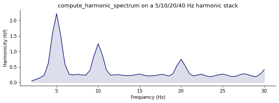
2. H-only spectrum (single signal)

For just the harmonicity factor H(f) — without the full PC and R computation — use compute_harmonic_spectrum. Returns the spectrum plus a rich complexity summary dict.

sig = harmonic_signal()

freqs, H, S, summary = compute_harmonic_spectrum(
    sig, precision_hz=0.5, fmin=2, fmax=30, fs=SF,
)

print("H shape:", H.shape)
print("S (kernel matrix) shape:", S.shape)
print("summary keys:", sorted(summary.keys()))
print("flatness:", summary['flatness'])
print("entropy:", summary['entropy'])
print("peaks:", summary['peaks'])

fig, ax = plt.subplots(figsize=(10, 3))
ax.plot(freqs, H, color='#1a237e')
ax.fill_between(freqs, 0, H, color='#1a237e', alpha=0.15)
ax.set_xlabel("Frequency (Hz)"); ax.set_ylabel("Harmonicity H(f)")
ax.set_title("compute_harmonic_spectrum on a 5/10/20/40 Hz harmonic stack")
plt.show()

H shape: (57,)
S (kernel matrix) shape: (57, 57)
summary keys: ['avg', 'entropy', 'flatness', 'higuchi', 'max', 'peak_harmsim', 'peak_harmsim_avg', 'peak_harmsim_max', 'peak_indices', 'peaks', 'peaks_avg', 'spread']
flatness: 0.7614612776395674
entropy: 5.358903605652942
peaks: [ 5. 10. 20.]

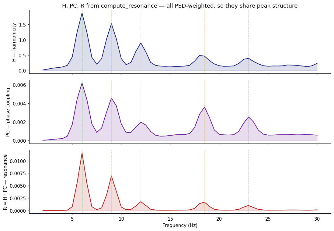
3. Full single-signal resonance R = H × PC

compute_resonance runs the full pipeline: harmonic kernel → ratio kernel → phase estimator → coupling metric → reducers → combine.

Important caveat: H, PC, R correlate by construction

Both H(f) and PC(f) are PSD-weighted in the orchestrator:

H(f)  = p(f) · Σⱼ S[f, j] · p(j)
PC(f) = p(f) · Σⱼ W[f, j] · Φ[f, j] · p(j)

So wherever PSD has a peak, both factors get amplified together — the raw spectra tend to share peak locations, just with different relative heights. To see whether peaks reflect real harmonic coupling vs broadband power, use surrogate normalization (Section 8) or compare against the same signal’s IAAFT-z-scored R.

We demonstrate this with the detuned_pair_signal, designed so the 9 + 18.5 Hz pair has nearly-identical PSD to the locked 6 + 12 Hz pair but NO actual phase coupling.

sig = detuned_pair_signal(duration=30.0)
cfg = ResonanceConfig(precision_hz=0.5, fmin=2, fmax=30, noverlap=900)
result = compute_resonance(sig, sf=SF, config=cfg)

print("type:", type(result).__name__)
print("freqs shape:", result.freqs.shape)
print("factors:", list(result.factors.keys()))
print("peaks:", result.peaks)
print()
print("Note that both H and PC peak at the 'detuned' site 9 Hz, not just")
print("the truly phase-locked site 6 Hz — this is the PSD-weighting effect.")
print()
print("Summaries (complexity per spectrum):")
for k, s in result.summaries.items():
    print(f"  {k}: flatness={s['flatness']:.3f}  entropy={s['entropy']:.3f}  "
          f"avg={s['avg']:.3g}")

type: ResonanceResult
freqs shape: (57,)
factors: ['H', 'PC']
peaks: {'H': array([ 6.,  9., 12.]), 'PC': array([ 6. ,  9. , 18.5, 23. , 12. ]), 'R': array([ 6. ,  9. , 12. , 18.5, 23. ])}

Note that both H and PC peak at the 'detuned' site 9 Hz, not just
the truly phase-locked site 6 Hz — this is the PSD-weighting effect.

Summaries (complexity per spectrum):
  H: flatness=0.678  entropy=5.244  avg=0.355
  PC: flatness=0.658  entropy=5.305  avg=0.00136
  R: flatness=0.229  entropy=4.091  avg=0.000941

# Getting different views of the result — the public API
print("Reduced 1-D spectra (length n_freqs):")
print(f"  result.factors['H'].shape          = {result.factors['H'].shape}")
print(f"  result.factors['PC'].shape         = {result.factors['PC'].shape}")
print(f"  result.resonance_spectrum.shape    = {result.resonance_spectrum.shape}")
print()
print("Per-spectrum scalar metrics (legacy compute_global_harmonicity columns):")
for k in ['H', 'PC', 'R']:
    s = result.summaries[k]
    print(f"  result.summaries[{k!r}]: avg={s['avg']:.3g}  max={s['max']:.3g}  "
          f"flatness={s['flatness']:.3f}  entropy={s['entropy']:.3f}  "
          f"spread={s['spread']:.3f}  peaks_avg={s['peaks_avg']:.2f}")
print()
print("Peak frequencies per spectrum:")
for k in ['H', 'PC', 'R']:
    print(f"  result.peaks[{k!r}] = {result.peaks[k]}")
print()
print("To get a flat pandas DataFrame across multiple results (legacy layout):")
print("  from biotuner.resonance import results_to_dataframe")
print("  df = results_to_dataframe([result, ...])   # 41 columns")
print()
print("Full N x N matrices (need return_intermediates=True on the config):")
print(f"  result.harmonicity_matrix   - raises AttributeError when not opted in,")
print(f"                                else (n_freqs, n_freqs) S[i, j]")
print(f"  result.phase_coupling_matrix - same, Phi[i, j]")

Reduced 1-D spectra (length n_freqs):
  result.factors['H'].shape          = (57,)
  result.factors['PC'].shape         = (57,)
  result.resonance_spectrum.shape    = (57,)

Per-spectrum scalar metrics (legacy compute_global_harmonicity columns):
  result.summaries['H']: avg=0.355  max=1.87  flatness=0.678  entropy=5.244  spread=7.169  peaks_avg=9.00
  result.summaries['PC']: avg=0.00136  max=0.00619  flatness=0.658  entropy=5.305  spread=7.314  peaks_avg=13.70
  result.summaries['R']: avg=0.000941  max=0.0116  flatness=0.229  entropy=4.091  spread=5.566  peaks_avg=13.70

Peak frequencies per spectrum:
  result.peaks['H'] = [ 6.  9. 12.]
  result.peaks['PC'] = [ 6.   9.  18.5 23.  12. ]
  result.peaks['R'] = [ 6.   9.  12.  18.5 23. ]

To get a flat pandas DataFrame across multiple results (legacy layout):
  from biotuner.resonance import results_to_dataframe
  df = results_to_dataframe([result, ...])   # 41 columns

Full N x N matrices (need return_intermediates=True on the config):
  result.harmonicity_matrix   - raises AttributeError when not opted in,
                                else (n_freqs, n_freqs) S[i, j]
  result.phase_coupling_matrix - same, Phi[i, j]

freqs = result.freqs
H = result.factors['H']; PC = result.factors['PC']; R = result.resonance_spectrum

fig, axes = plt.subplots(3, 1, figsize=(10, 7), sharex=True)
for ax, (name, vals, color) in zip(axes, [
    ('H — harmonicity',           H,  '#1a237e'),
    ('PC — phase coupling',       PC, '#6a1b9a'),
    ('R = H · PC — resonance',    R,  '#b71c1c'),
]):
    ax.plot(freqs, vals, color=color)
    ax.fill_between(freqs, 0, vals, color=color, alpha=0.15)
    ax.set_ylabel(name)
    for tgt, lbl, col in [(6, '6 (locked)', 'green'),
                            (9, '9 (detuned)', 'orange'),
                            (12, '12 (locked)', 'green'),
                            (18.5, '18.5 (detuned)', 'orange'),
                            (23, '23 (lone)', 'red')]:
        ax.axvline(tgt, color=col, alpha=0.4, lw=0.7, ls='--')

axes[-1].set_xlabel("Frequency (Hz)")
axes[0].set_title("H, PC, R from compute_resonance — all PSD-weighted, so they share peak structure")
plt.tight_layout(); plt.show()

# Quantify how similar H/PC/R shapes are (Pearson correlation, normalized to max)
print()
def corr(a, b): return float(np.corrcoef(a/a.max(), b/b.max())[0, 1])
print("Shape correlations (peak-aligned across spectra):")
print(f"  H ~ PC = {corr(H, PC):.3f}")
print(f"  H ~ R  = {corr(H, R):.3f}")
print(f"  PC ~ R = {corr(PC, R):.3f}")
print()
print("Both H and PC are PSD-weighted in the orchestrator (Step 9 reducer:")
print("v[i] = p[i] * sum_j M[i,j] * p[j]), so wherever PSD peaks, both factors")
print("are amplified. To distinguish TRUE phase coupling from PSD-impostors,")
print("use surrogate normalization (Section 8) — AAFT/IAAFT surrogates preserve")
print("PSD but destroy phase relations, so the z-scored R isolates pure coupling.")

Shape correlations (peak-aligned across spectra):
  H ~ PC = 0.933
  H ~ R  = 0.952
  PC ~ R = 0.907

Both H and PC are PSD-weighted in the orchestrator (Step 9 reducer:
v[i] = p[i] * sum_j M[i,j] * p[j]), so wherever PSD peaks, both factors
are amplified. To distinguish TRUE phase coupling from PSD-impostors,
use surrogate normalization (Section 8) — AAFT/IAAFT surrogates preserve
PSD but destroy phase relations, so the z-scored R isolates pure coupling.

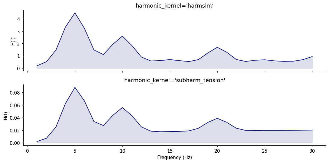
4. Swapping harmonic kernels

Two harmonic kernels are registered: harmsim (Gill-Purves dyad similarity) and subharm_tension (Chan subharmonic tension, inverted). They give qualitatively similar peak structure but differ in absolute magnitude and how strongly they penalize complex ratios.

sig = harmonic_signal()

results = {}
for kernel in ['harmsim', 'subharm_tension']:
    cfg = ResonanceConfig(harmonic_kernel=kernel)
    results[kernel] = compute_resonance(sig, sf=SF, config=cfg)

fig, axes = plt.subplots(2, 1, figsize=(10, 5), sharex=True)
for ax, (kernel, r) in zip(axes, results.items()):
    ax.plot(r.freqs, r.factors['H'], color='#1a237e', label='H(f)')
    ax.fill_between(r.freqs, 0, r.factors['H'], color='#1a237e', alpha=0.15)
    ax.set_title(f"harmonic_kernel='{kernel}'")
    ax.set_ylabel('H(f)')
axes[-1].set_xlabel("Frequency (Hz)")
plt.tight_layout(); plt.show()

C:\Users\skite\Documents\Github\biotuner\.claude\worktrees\sweet-hamilton-6c0f0d\biotuner\metrics.py:954: RuntimeWarning: divide by zero encountered in scalar divide
  harm_temp.append(1 / delta_norm)

5. Coupling metrics — and the n:m convention rule

Six pairwise metrics are registered, falling into two input-type categories:

• phase inputs: nm_plv, nm_pli, nm_wpli, nm_rrci, nm_plv_canonical.

• analytic inputs: nm_wpli_complex.

Important: convention rule

All ratio kernels in biotuner (binary, fraction, future Arnold-tongue) return (n, m) with the convention ratio = f_j / f_i = m / n. The plain nm_plv applies this as n·φ_i − m·φ_j, which is mathematically wrong for true n:m phase locking under Tass 1998. For correct n:m phase-coupling tests, use coupling_metric='nm_plv_canonical' — it swaps (n, m) internally to apply the Tass formula. nm_plv is kept for bit-exact reproduction of legacy paper analyses only.

Where do these metrics actually differ?

For long, clean, single-signal data, all phase-input metrics give similar PC shapes (because they all measure the same underlying STFT phase coherence, just with different rejection of common-mode components). To see the theoretical differences cleanly, apply the metrics directly to synthesized phase arrays representing three canonical coupling regimes:

from biotuner.resonance.coupling import nm_plv, nm_pli, nm_wpli, nm_plv_canonical, nm_rrci

# Synthesize per-window phase arrays under three canonical coupling regimes
rng = np.random.default_rng(0)
N = 5000
phi_a = 2 * np.pi * rng.random(N)

regimes = {
    'zero_lag (0)':       phi_a.copy(),                          # identical phases
    'lagged (pi/3)':      phi_a + np.pi / 3,                     # constant offset
    'anti_phase (pi)':    phi_a + np.pi,                         # anti-aligned
    'noisy_lag':          phi_a + np.pi / 3 + 0.6 * rng.standard_normal(N),
    'uncoupled':          2 * np.pi * rng.random(N),             # independent
}

metrics = {
    'PLV':              nm_plv,
    'PLV_canonical':    nm_plv_canonical,
    'PLI':              nm_pli,
    'wPLI':             nm_wpli,
    'RRCi':             nm_rrci,
}

# Compute and tabulate
print(f"{'regime':<22}  " + "  ".join(f"{name:>14}" for name in metrics))
print("-" * (22 + len(metrics) * 16))
results = {}
for regime, phi_b in regimes.items():
    row = {}
    for mname, mfn in metrics.items():
        row[mname] = mfn(phi_a, phi_b, 1, 1)
    results[regime] = row
    print(f"{regime:<22}  " + "  ".join(f"{row[n]:>14.4f}" for n in metrics))
print()
print("Key observations:")
print("  PLV peaks for zero_lag AND lagged (it sees ALL constant phase relations)")
print("  PLI/wPLI ~ 0 for zero_lag and anti_phase (sin(Delta phi) = 0)")
print("  PLI/wPLI peak for lagged (Delta phi = pi/3 gives nonzero imag part)")
print("  All metrics ~ 0 for uncoupled (random phase difference)")

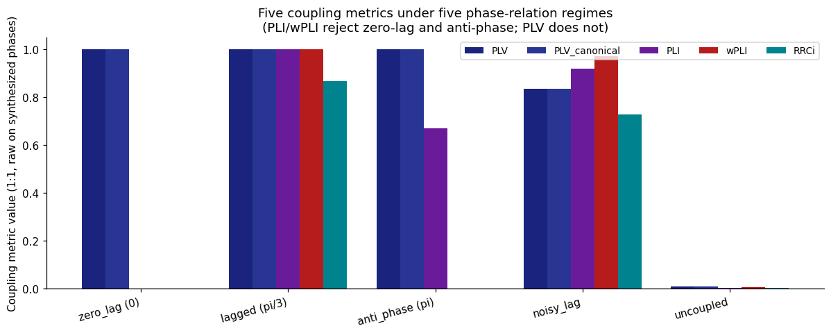
regime                             PLV   PLV_canonical             PLI            wPLI            RRCi
------------------------------------------------------------------------------------------------------
zero_lag (0)                    1.0000          1.0000          0.0000          0.0000          0.0000
lagged (pi/3)                   1.0000          1.0000          1.0000          1.0000          0.8660
anti_phase (pi)                 1.0000          1.0000          0.6708          0.0000          0.0000
noisy_lag                       0.8343          0.8343          0.9196          0.9708          0.7286
uncoupled                       0.0081          0.0081          0.0024          0.0069          0.0044

Key observations:
  PLV peaks for zero_lag AND lagged (it sees ALL constant phase relations)
  PLI/wPLI ~ 0 for zero_lag and anti_phase (sin(Delta phi) = 0)
  PLI/wPLI peak for lagged (Delta phi = pi/3 gives nonzero imag part)
  All metrics ~ 0 for uncoupled (random phase difference)

# Grouped bar plot of the same table
fig, ax = plt.subplots(figsize=(11, 4.5))
regime_names = list(regimes)
x = np.arange(len(regime_names))
width = 0.16
colors = ['#1a237e', '#283593', '#6a1b9a', '#b71c1c', '#00838f']
for i, (mname, color) in enumerate(zip(metrics, colors)):
    vals = [results[r][mname] for r in regime_names]
    ax.bar(x + (i - len(metrics)/2 + 0.5) * width, vals, width, label=mname, color=color)
ax.set_xticks(x); ax.set_xticklabels(regime_names, rotation=15, ha='right')
ax.set_ylabel("Coupling metric value (1:1, raw on synthesized phases)")
ax.set_title("Five coupling metrics under five phase-relation regimes\n"
              "(PLI/wPLI reject zero-lag and anti-phase; PLV does not)")
ax.legend(loc='upper right', ncols=5, fontsize=9)
ax.set_ylim(0, 1.05)
plt.tight_layout(); plt.show()

6. Ratio kernels — binary (legacy) vs fraction (new)

The ratio kernel decides which (n, m) integer pair to test at each frequency pair, and how heavily to weight the result.

• binary — iterates 1 ≤ n, m ≤ max_nm (default 3), picks the best match within 5% tolerance. Returns W=1 if matched, W=0 otherwise — or (n=1, m=1) if fallback_to_1_1=True. Misses any ratio outside the small preset table.

• fraction — computes Fraction(f_j / f_i).limit_denominator(max_denom) to find the EXACT closest rational. Weights via Tenney height W = exp(-β · log₂(n·m)), so simple ratios dominate but complex ones can still be tested.

Demonstration: a 10 + 17 Hz phase-locked signal

17 / 10 = 1.7 matches no integer ratio with n, m ≤ 3, so binary falls back to 1:1 (testing a meaningless 10:10 coupling at the 10/17 bin pair). fraction returns (n=10, m=17) — the actual mode-lock — though heavily down-weighted by Tenney height.

# Build a 10:17 phase-locked signal
def lock_signal_1017(sf=SF, duration=30.0, seed=0):
    n = int(sf * duration); t = np.arange(n) / sf
    phi_unit = 2 * np.pi * 1.0 * t  # common subharmonic
    # 10 Hz and 17 Hz share the same 1 Hz base phase — true 10:17 lock
    sig = (np.sin(10 * phi_unit) + 0.7 * np.sin(17 * phi_unit + 0.3)
           + 0.15 * pink_noise(n, sf, seed=seed))
    return sig

sig_1017 = lock_signal_1017()

print("Ratio kernel comparison at the 10 Hz peak:")
print(f"{'kernel':<10}  {'PC(10)':>8}  {'PC(17)':>8}  {'(n, m) at (10, 17)':<22}")
print("-" * 60)

import numpy as _np
for kernel_name, kernel_params in [
    ('binary',  {'max_nm': 3, 'tolerance': 0.05, 'fallback_to_1_1': True}),
    ('fraction', {'max_denom': 32, 'beta': 0.5}),
]:
    cfg = ResonanceConfig(
        precision_hz=0.5, fmin=2, fmax=30, noverlap=900,
        ratio_kernel=kernel_name,
        ratio_kernel_params=kernel_params,
        coupling_metric='nm_plv_canonical',  # always pair with canonical
    )
    r = compute_resonance(sig_1017, sf=SF, config=cfg)
    i10 = int(_np.argmin(_np.abs(r.freqs - 10)))
    i17 = int(_np.argmin(_np.abs(r.freqs - 17)))

    # Probe what (n, m) the kernel actually returned at (10, 17)
    from biotuner.resonance.registry import RATIO_KERNELS
    W, N, M = RATIO_KERNELS[kernel_name](_np.array([10.0]), _np.array([17.0]),
                                          **kernel_params)
    nm_str = f"n={int(N[0,0])}, m={int(M[0,0])}, W={W[0,0]:.3f}"

    print(f"{kernel_name:<10}  {r.factors['PC'][i10]:>8.4f}  {r.factors['PC'][i17]:>8.4f}  {nm_str}")

print()
print("Reading: binary maps (10, 17) -> (n=1, m=1) — a spurious 1:1 test that")
print("contaminates the PC sum with whatever bins look 1:1 to 10 Hz.")
print("fraction maps (10, 17) -> (n=10, m=17) — the TRUE mode-lock — with a")
print("small Tenney weight reflecting how complex the ratio is.")

Ratio kernel comparison at the 10 Hz peak:
kernel        PC(10)    PC(17)  (n, m) at (10, 17)    
------------------------------------------------------------
binary        0.0249    0.0080  n=1, m=1, W=1.000

fraction      0.0003    0.0002  n=10, m=17, W=0.025

Reading: binary maps (10, 17) -> (n=1, m=1) — a spurious 1:1 test that
contaminates the PC sum with whatever bins look 1:1 to 10 Hz.
fraction maps (10, 17) -> (n=10, m=17) — the TRUE mode-lock — with a
small Tenney weight reflecting how complex the ratio is.

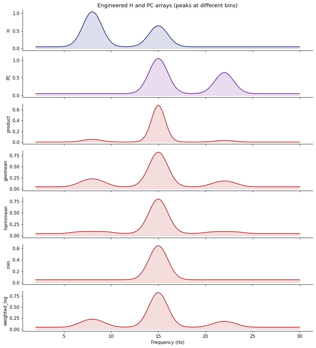
7. Combine rules — H × PC → R

Five combine rules. Default product (R = H · PC) is the legacy semantics.

For typical signals from compute_resonance (where H and PC are PSD-weighted and end up with similar shapes), the five combine rules look very similar to each other. To make their differences visible, we construct a synthetic (H_arr, PC_arr) pair where peaks live at DIFFERENT bins, and apply each combine rule directly.

from biotuner.resonance.registry import COMBINE_RULES

# Construct H and PC with peaks at DIFFERENT frequencies on purpose
freqs = np.linspace(2, 30, 200)
def gauss(c, w, h): return h * np.exp(-((freqs - c) ** 2) / (2 * w ** 2))

H_arr  = gauss(8,  1.0, 1.0) + gauss(15, 1.0, 0.6) + 0.05      # peaks at 8, 15
PC_arr = gauss(15, 1.0, 1.0) + gauss(22, 1.0, 0.6) + 0.05      # peaks at 15, 22

print("Peaks: H at 8 & 15 ; PC at 15 & 22.")
print("Combine rules respond DIFFERENTLY to non-overlapping peaks:")
print()

fig, axes = plt.subplots(7, 1, figsize=(10, 11), sharex=True)
axes[0].plot(freqs, H_arr, color='#1a237e', label='H'); axes[0].fill_between(freqs, 0, H_arr, color='#1a237e', alpha=0.15)
axes[0].set_ylabel('H'); axes[0].set_title('Engineered H and PC arrays (peaks at different bins)')
axes[1].plot(freqs, PC_arr, color='#6a1b9a', label='PC'); axes[1].fill_between(freqs, 0, PC_arr, color='#6a1b9a', alpha=0.15)
axes[1].set_ylabel('PC')

for ax, rule_name in zip(axes[2:], ['product', 'geomean', 'harmmean', 'min', 'weighted_log']):
    rule = COMBINE_RULES[rule_name]
    R_arr = rule([H_arr, PC_arr])
    ax.plot(freqs, R_arr, color='#b71c1c')
    ax.fill_between(freqs, 0, R_arr, color='#b71c1c', alpha=0.15)
    ax.set_ylabel(rule_name)

axes[-1].set_xlabel("Frequency (Hz)")

# Annotate where each combine rule places its peak
peak_freqs = {}
for rule_name in ['product', 'geomean', 'harmmean', 'min', 'weighted_log']:
    R_arr = COMBINE_RULES[rule_name]([H_arr, PC_arr])
    peak_freqs[rule_name] = freqs[int(np.argmax(R_arr))]
plt.tight_layout(); plt.show()

print()
print("Peak frequency of R(f) per rule:")
for rule_name, pf in peak_freqs.items():
    print(f"  {rule_name:<15}  {pf:.2f} Hz")
print()
print("'min' and 'harmmean' aggressively reject sites where one factor is small:")
print("  peak settles at 15 (the only overlap).")
print("'product'/'geomean' tilt toward 15 but preserve some signal at 8 (H high)")
print("  and 22 (PC high). 'weighted_log' further amplifies asymmetry.")

Peaks: H at 8 & 15 ; PC at 15 & 22.
Combine rules respond DIFFERENTLY to non-overlapping peaks:

Peak frequency of R(f) per rule:
  product          14.94 Hz
  geomean          14.94 Hz
  harmmean         14.94 Hz
  min              14.94 Hz
  weighted_log     14.94 Hz

'min' and 'harmmean' aggressively reject sites where one factor is small:
  peak settles at 15 (the only overlap).
'product'/'geomean' tilt toward 15 but preserve some signal at 8 (H high)
  and 22 (PC high). 'weighted_log' further amplifies asymmetry.

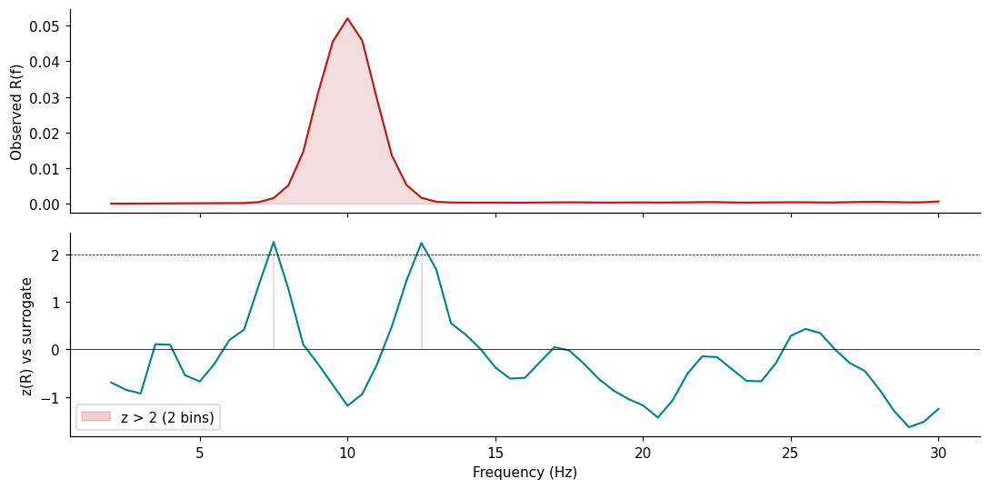
8. Surrogate-null normalization

For statistical inference, with_surrogate_null runs the resonance pipeline on the observed signal AND on n AAFT/phase-randomized surrogates, then z-scores the observed against the surrogate distribution.

For a noisy alpha-burst signal, the surrogates destroy phase structure while preserving PSD — so high z-scores at the alpha carrier are evidence of true phase-locked alpha, not just elevated PSD.

sig = alpha_burst_signal()

cfg = ResonanceConfig(precision_hz=0.5, fmin=2, fmax=30)
result_z = with_surrogate_null(
    sig, sf=SF, config=cfg, surr_type='AAFT', n=50, correction='both', parallel=False,
)

freqs = result_z.freqs
R = result_z.resonance_spectrum
z = result_z.resonance_spectrum_z

fig, axes = plt.subplots(2, 1, figsize=(10, 5), sharex=True)
axes[0].plot(freqs, R, color='#b71c1c')
axes[0].fill_between(freqs, 0, R, color='#b71c1c', alpha=0.15)
axes[0].set_ylabel("Observed R(f)")

axes[1].plot(freqs, z, color='#00838f')
axes[1].axhline(0, color='k', lw=0.5); axes[1].axhline(2, color='k', ls='--', lw=0.5)
sig_mask = z > 2
if sig_mask.any():
    axes[1].fill_between(freqs, 0, z, where=sig_mask, color='#b71c1c', alpha=0.2,
                          label=f"z > 2 ({sig_mask.sum()} bins)")
    axes[1].legend()
axes[1].set_ylabel("z(R) vs surrogate")
axes[1].set_xlabel("Frequency (Hz)")
plt.tight_layout(); plt.show()

9. Cross-channel resonance — compute_cross_resonance

The cross-channel analog of compute_resonance, for two signals. Returns a CrossResonanceResult with three reducer flavors per factor:

• '1to2' — asymmetric (signal1 at i, signal2 at j)

• '2to1' — transposed

• 'all' — symmetrized average

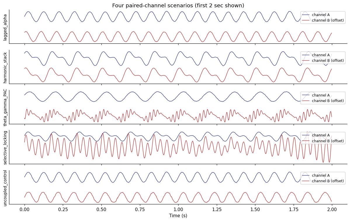
The three flavors expose directional information that the symmetric average loses. We’ll work through four progressively richer paired-channel cases.

9a. Four paired-channel scenarios

The same compute_cross_resonance(sig1, sig2) call applies to all of them — only the input changes.

# Build four paired-channel datasets covering different coupling regimes.
SCENARIO_DUR = 12.0   # seconds
SCENARIO_T   = np.arange(int(SF * SCENARIO_DUR)) / SF

def _noise(seed, scale=0.2):
    return scale * pink_noise(len(SCENARIO_T), SF, seed=seed)

def alpha_lagged(seed=0):
    """Same 10 Hz in both channels, B lags A by pi/3. Simple lagged coupling."""
    t = SCENARIO_T
    phi = 2 * np.pi * 10 * t
    return np.sin(phi) + _noise(seed + 1), np.sin(phi + np.pi/3) + _noise(seed + 2)

def harmonic_stack_xchan(seed=0):
    """6+12 Hz phase-locked harmonic stack in both channels, B offset by pi/8.
    Rich harmonic coupling — H, PC, R all peak at both 6 and 12 Hz."""
    t = SCENARIO_T
    phi = 2 * np.pi * 6 * t + 0.4
    a = 1.2 * np.sin(phi) + 0.7 * np.sin(2 * phi + 0.3) + _noise(seed + 1)
    b = 1.2 * np.sin(phi + np.pi/8) + 0.7 * np.sin(2 * phi + 0.3 + np.pi/8) + _noise(seed + 2)
    return a, b

def theta_gamma_pac(seed=0):
    """Theta-gamma cross-frequency coupling.
    A: clean 6 Hz theta.
    B: 6 Hz theta + 40 Hz gamma amplitude-modulated by the theta phase
       (gamma is loudest at theta peaks). The two share a base frequency,
       but B carries an additional cross-frequency 6:40 amplitude lock."""
    t = SCENARIO_T
    rng = np.random.default_rng(seed)
    theta = np.sin(2 * np.pi * 6 * t + 0.3)
    a = theta + _noise(seed + 1)
    # gamma envelope follows theta amplitude (peaks at theta peaks)
    gamma_env = 0.5 * (1 + np.cos(2 * np.pi * 6 * t + 0.3))   # 0..1, locked to theta
    gamma = gamma_env * np.sin(2 * np.pi * 40 * t + rng.uniform(0, 2*np.pi))
    b = 0.7 * theta + 1.0 * gamma + _noise(seed + 2)
    return a, b

def uncoupled_control(seed=0):
    """Independent 10 Hz oscillators with random-walk phase drift in B."""
    t = SCENARIO_T; rng = np.random.default_rng(seed)
    a = np.sin(2 * np.pi * 10 * t) + _noise(seed + 1)
    dphi = rng.standard_normal(len(t)) * 1.0 * np.sqrt(1.0/SF)
    b = np.sin(2 * np.pi * 10 * t + np.cumsum(dphi)) + _noise(seed + 2)
    return a, b

def selective_locking(seed=0):
    """Designed so H peaks WHERE PC DOES NOT — three PSD peaks, only one
    actually phase-locked across channels.

    Both channels share a 6+12 Hz phase-locked harmonic stack (so PC should
    peak at 6 and 12). Channel B has an ADDITIONAL narrowband-noise component
    centered at 24 Hz (a strong PSD peak, but its phase is independent of A
    since it's driven by white noise). The 24 Hz peak is a 1:2 partner of 12
    Hz in PSD space, so H gets a contribution there — but the phase coupling
    is absent, so PC at 24 Hz is low.

    Expected:  H peaks at 6, 12, AND 24
               PC peaks at 6 and 12 only
    """
    from scipy.signal import butter, filtfilt
    t = SCENARIO_T; rng = np.random.default_rng(seed)
    phi = 2 * np.pi * 6 * t
    a = 1.2 * np.sin(phi) + 0.8 * np.sin(2 * phi + 0.3) + _noise(seed + 1)
    b_locked = 1.2 * np.sin(phi + np.pi/6) + 0.8 * np.sin(2 * phi + 0.3 + np.pi/6)
    # Narrowband noise centered at 24 Hz — strong PSD peak, random phase per window
    w = rng.standard_normal(len(t))
    nyq = SF / 2; bw_hz = 1.0
    bcoef, acoef = butter(4, [(24 - bw_hz/2)/nyq, (24 + bw_hz/2)/nyq], btype='band')
    noise_24 = filtfilt(bcoef, acoef, w); noise_24 /= noise_24.std()
    b = b_locked + 2.5 * noise_24 + _noise(seed + 2)
    return a, b

SCENARIOS = {
    'lagged_alpha':       alpha_lagged(),
    'harmonic_stack':     harmonic_stack_xchan(),
    'theta_gamma_PAC':    theta_gamma_pac(),
    'selective_locking':  selective_locking(),
    'uncoupled_control':  uncoupled_control(),
}

# Plot waveforms (first 2 sec) for each pair
fig, axes = plt.subplots(len(SCENARIOS), 1, figsize=(11, 7), sharex=True)
t_show = SCENARIO_T[:int(SF * 2)]
for ax, (name, (a, b)) in zip(axes, SCENARIOS.items()):
    ax.plot(t_show, a[:len(t_show)], color='#1a237e', lw=0.8, label='channel A')
    ax.plot(t_show, b[:len(t_show)] - 4, color='#b71c1c', lw=0.8, label='channel B (offset)')
    ax.set_ylabel(name, fontsize=9)
    ax.set_yticks([]); ax.legend(loc='upper right', fontsize=8)
axes[-1].set_xlabel("Time (s)")
axes[0].set_title("Four paired-channel scenarios (first 2 sec shown)")
plt.tight_layout(); plt.show()

9b. Cross-resonance R(f) compared across all four scenarios

cfg_xc = ResonanceConfig(precision_hz=0.5, fmin=2, fmax=50, noverlap=400)

results = {}
for name, (a, b) in SCENARIOS.items():
    results[name] = compute_cross_resonance(a, b, sf=SF, config=cfg_xc)

# Stacked H / PC / R panel comparison (symmetric 'all' flavor)
fig, axes = plt.subplots(3, 1, figsize=(11, 7), sharex=True)
colors = ['#1a237e', '#2e7d32', '#b71c1c', '#ef6c00', '#7d7d7d']
for ax, (lbl, factor_key) in zip(axes, [
    ('H — harmonicity',      'H'),
    ('PC — phase coupling',  'PC'),
    ('R = H · PC',           None),  # None means resonance_spectrum
]):
    for (name, r), color in zip(results.items(), colors):
        vals = r.resonance_spectrum['all'] if factor_key is None else r.factors[factor_key]['all']
        ax.plot(r.freqs, vals, label=name, color=color, lw=1.4)
    ax.set_ylabel(lbl)
    ax.legend(loc='upper right', fontsize=8, ncols=3)
axes[-1].set_xlabel("Frequency (Hz)")
axes[0].set_title("Cross-channel H / PC / R across coupling regimes — note for 'selective_locking', H peaks at 24 Hz\n"
                   "(narrowband-noise impostor with simple-ratio PSD partners) while PC does NOT")
plt.tight_layout(); plt.show()

# Numeric table: which frequencies dominate H vs PC vs R, per scenario?
print()
print(f"{'scenario':<22}  {'top H peak':>16}  {'top PC peak':>16}  {'top R peak':>16}")
print("-" * 75)
for name, r in results.items():
    H = r.factors['H']['all']
    PC = r.factors['PC']['all']
    R = r.resonance_spectrum['all']
    f_H  = r.freqs[int(np.argmax(H))]
    f_PC = r.freqs[int(np.argmax(PC))]
    f_R  = r.freqs[int(np.argmax(R))]
    print(f"{name:<22}  {f'{f_H:.1f} Hz ({H.max():.3f})':>16}  "
          f"{f'{f_PC:.1f} Hz ({PC.max():.3f})':>16}  "
          f"{f'{f_R:.1f} Hz ({R.max():.3f})':>16}")
print()
print("For 'selective_locking', H's 24 Hz contribution from the narrowband-noise")
print("impostor is visible — PC tells the truth: no actual coupling there.")

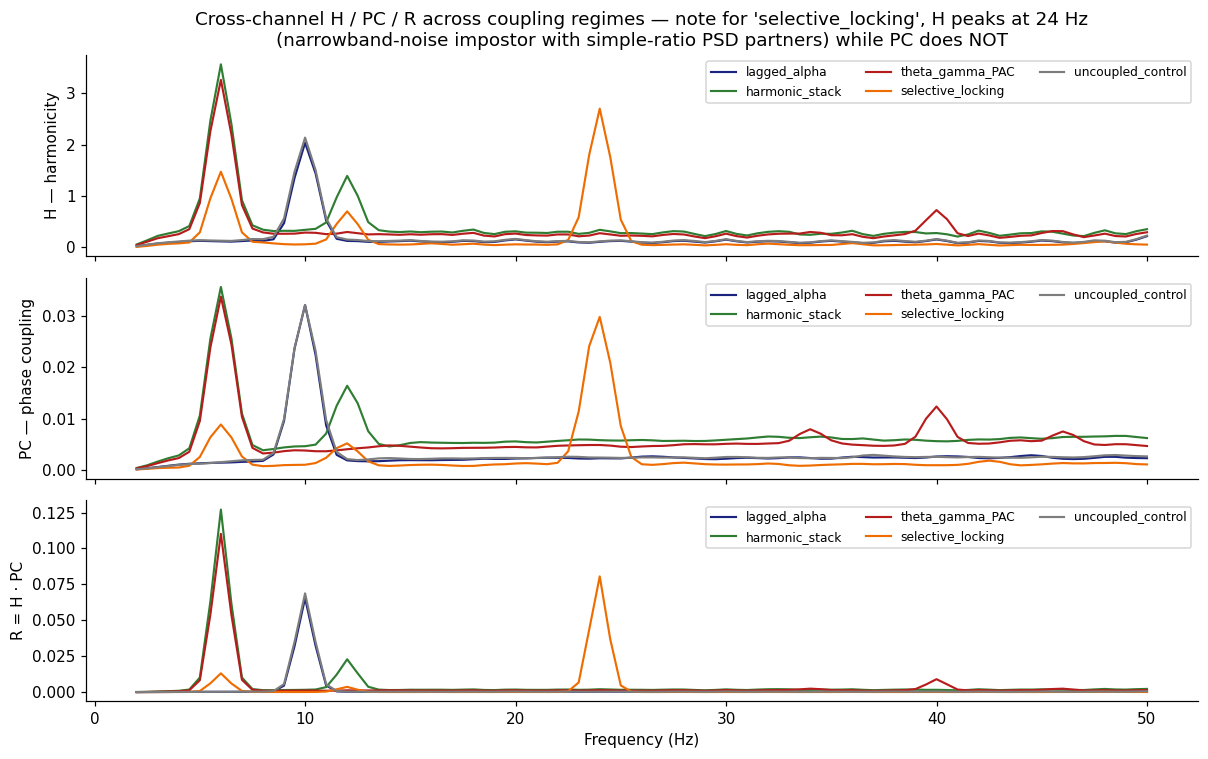
scenario                      top H peak       top PC peak        top R peak
---------------------------------------------------------------------------
lagged_alpha             10.0 Hz (2.038)   10.0 Hz (0.032)   10.0 Hz (0.065)
harmonic_stack            6.0 Hz (3.567)    6.0 Hz (0.036)    6.0 Hz (0.127)
theta_gamma_PAC           6.0 Hz (3.265)    6.0 Hz (0.034)    6.0 Hz (0.110)
selective_locking        24.0 Hz (2.703)   24.0 Hz (0.030)   24.0 Hz (0.081)
uncoupled_control        10.0 Hz (2.140)   10.0 Hz (0.032)   10.0 Hz (0.069)

For 'selective_locking', H's 24 Hz contribution from the narrowband-noise
impostor is visible — PC tells the truth: no actual coupling there.

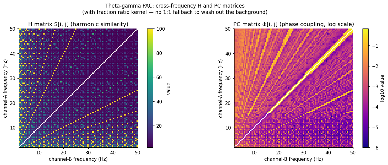
9c. Cross-resonance MATRICES — what the spectra throw away

The H(f) and PC(f) spectra are reductions of the full N × N cross-frequency matrices, where entry [i, j] = (similarity / phase coupling) between channel-1 frequency bin i and channel-2 frequency bin j. The spectra collapse columns away. For diagnostics — and especially for cross-frequency coupling — it pays to inspect the matrices directly via result.intermediates.

# Re-run on theta-gamma PAC with the FRACTION ratio kernel.
# This is important: the default 'binary' kernel with fallback_to_1_1=True
# fills Phi[i,j] for EVERY frequency pair (testing 1:1 coupling at non-matching
# pairs), which washes out the heatmap. The 'fraction' kernel returns the
# exact (n, m) for the closest rational and weights via Tenney height — so
# simple-ratio cells stand out cleanly against an exponentially suppressed
# background of complex ratios.
a, b = SCENARIOS['theta_gamma_PAC']
cfg_keep = ResonanceConfig(
    precision_hz=0.5, fmin=2, fmax=50, noverlap=400,
    ratio_kernel='fraction',
    ratio_kernel_params={'max_denom': 16, 'beta': 1.0},
    coupling_metric='nm_plv_canonical',
    return_intermediates=True,
)
r_pac = compute_cross_resonance(a, b, sf=SF, config=cfg_keep)
# With return_intermediates=True, the N×N matrices are accessible as typed
# properties on the result — no dictionary fishing required.
H_mat  = r_pac.harmonicity_matrix
PC_mat = r_pac.phase_coupling_matrix
print(f"H matrix shape:  {H_mat.shape}")
print(f"PC matrix shape: {PC_mat.shape}")

freqs = r_pac.freqs

def _heatmap(ax, M, title, cmap='viridis', vmax=None, log=False):
    M_show = M.copy().astype(float)
    np.fill_diagonal(M_show, np.nan)                     # mask self-pair
    if log:
        # log scale for highly skewed Tenney-weighted matrix
        with np.errstate(divide='ignore'):
            M_show = np.log10(np.clip(M_show, 1e-6, None))
        cb_label = 'log10 value'
    else:
        cb_label = 'value'
    finite = M_show[np.isfinite(M_show)]
    vmin = float(np.nanmin(finite)) if finite.size else 0.0
    if vmax is None:
        vmax = float(np.nanmax(finite)) if finite.size else 1.0
    im = ax.imshow(M_show, origin='lower', cmap=cmap, aspect='equal',
                    vmin=vmin, vmax=vmax,
                    extent=[freqs[0], freqs[-1], freqs[0], freqs[-1]])
    ax.set_xlabel('channel-B frequency (Hz)')
    ax.set_ylabel('channel-A frequency (Hz)')
    ax.set_title(title)
    plt.colorbar(im, ax=ax, fraction=0.046, label=cb_label)

fig, axes = plt.subplots(1, 2, figsize=(13, 5))
_heatmap(axes[0], H_mat,  'H matrix S[i, j] (harmonic similarity)',          cmap='viridis')
_heatmap(axes[1], PC_mat, 'PC matrix Φ[i, j] (phase coupling, log scale)',   cmap='plasma', log=True)
fig.suptitle('Theta-gamma PAC: cross-frequency H and PC matrices\n'
              '(with fraction ratio kernel — no 1:1 fallback to wash out the background)',
              fontsize=11)
plt.tight_layout(); plt.show()
print()
print("Reading the H matrix: bright cells line up along simple-ratio bands radiating")
print("from the diagonal (the 1:2 ridge, 1:3 ridge, etc.) — that's the harmonic")
print("similarity grid. The diagonal is masked.")
print()
print("Reading the PC matrix (log10): the dominant hot spot is the (6 Hz, 12 Hz)")
print("region where the shared theta drives a 1:2 phase lock. The vertical band")
print("around 40 Hz on channel B shows cross-frequency phase coupling between")
print("channel A's theta and channel B's gamma envelope — the theta-gamma PAC.")

H matrix shape:  (97, 97)
PC matrix shape: (97, 97)

Reading the H matrix: bright cells line up along simple-ratio bands radiating
from the diagonal (the 1:2 ridge, 1:3 ridge, etc.) — that's the harmonic
similarity grid. The diagonal is masked.

Reading the PC matrix (log10): the dominant hot spot is the (6 Hz, 12 Hz)
region where the shared theta drives a 1:2 phase lock. The vertical band
around 40 Hz on channel B shows cross-frequency phase coupling between
channel A's theta and channel B's gamma envelope — the theta-gamma PAC.

9d. Directional flavors — 1to2 vs 2to1 vs all

For an asymmetric coupling like theta-gamma PAC (channel B carries an extra cross-frequency lock that channel A does not), the three reducer flavors expose directional information that the symmetric 'all' average loses.

# Same theta-gamma PAC result
fig, axes = plt.subplots(3, 1, figsize=(11, 7), sharex=True)
for ax, (lbl, factor) in zip(axes, [
    ('H', 'H'), ('PC', 'PC'), ('R', None),
]):
    for flavor, ls, color in [('all', '-', '#37474f'),
                                ('1to2', '--', '#1a237e'),
                                ('2to1', ':',  '#b71c1c')]:
        vals = (r_pac.resonance_spectrum[flavor] if factor is None
                else r_pac.factors[factor][flavor])
        ax.plot(r_pac.freqs, vals, ls=ls, color=color, lw=1.4, label=flavor)
    ax.set_ylabel(lbl)
    ax.legend(loc='upper right', fontsize=9)
axes[-1].set_xlabel("Frequency (Hz)")
axes[0].set_title("Theta-gamma PAC: directional flavors of cross-resonance\n"
                   "1to2 weights channel A's PSD at f; 2to1 weights channel B's. "
                   "Their difference reveals which side drives which band.")
plt.tight_layout(); plt.show()

# Directional asymmetry index at key frequencies
print()
print("Directional asymmetry index (1to2 - 2to1) / (1to2 + 2to1):")
for f0 in [6, 12, 40]:
    i = int(np.argmin(np.abs(r_pac.freqs - f0)))
    a12 = r_pac.resonance_spectrum['1to2'][i]
    a21 = r_pac.resonance_spectrum['2to1'][i]
    denom = a12 + a21
    asym = (a12 - a21) / denom if denom > 0 else 0.0
    print(f"  {f0:>3} Hz   1to2={a12:.4f}  2to1={a21:.4f}  asymmetry={asym:+.3f}")

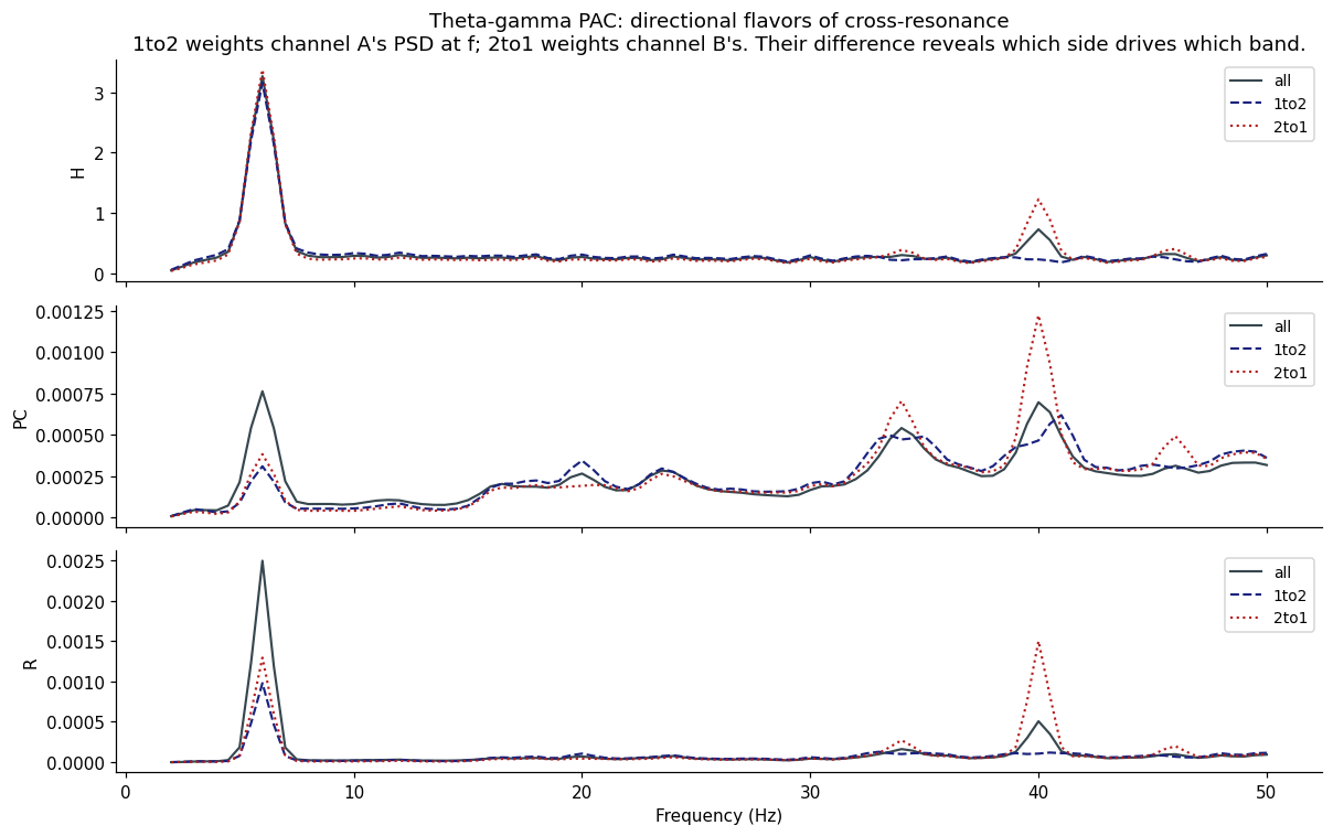
Directional asymmetry index (1to2 - 2to1) / (1to2 + 2to1):
    6 Hz   1to2=0.0010  2to1=0.0013  asymmetry=-0.139
   12 Hz   1to2=0.0000  2to1=0.0000  asymmetry=+0.249
   40 Hz   1to2=0.0001  2to1=0.0015  asymmetry=-0.868

9e. Surrogate-normalized cross-resonance

The same surrogate-normalization story as Section 8, applied to cross-channel data. Here, we use compute_cross_resonance_connectivity_zscore from the multi-channel API but on a 2-row matrix to make the comparison explicit: how much of the observed coupling survives a null that preserves each channel’s PSD but destroys their cross-channel phase relation?

# Use the harmonic-stack scenario (cleanest signal-vs-noise)
a, b = SCENARIOS['harmonic_stack']
data_2ch = np.stack([a, b])

hc2 = harmonic_connectivity(
    sf=SF, data=data_2ch, peaks_function='FOOOF',
    precision=0.5, n_harm=5, min_freq=2, max_freq=30, n_peaks=4,
)

obs, z, p = hc2.compute_cross_resonance_connectivity_zscore(
    config=cfg_xc, factor='R', flavor='all', aggregate='peak_to_median',
    surrogate_kind='iaaft', n_surrogates=20, rng_seed=42, graph=False,
)
print(f"Observed R aggregate (off-diagonal): {obs[0,1]:.4f}")
print(f"z-score vs IAAFT null:               {z[0,1]:.2f}")
print(f"Empirical p-value:                   {p[0,1]:.4f}")
print()

# Compare against uncoupled control
a, b = SCENARIOS['uncoupled_control']
data_2ch_uc = np.stack([a, b])
hc2_uc = harmonic_connectivity(
    sf=SF, data=data_2ch_uc, peaks_function='FOOOF',
    precision=0.5, n_harm=5, min_freq=2, max_freq=30, n_peaks=4,
)
obs2, z2, p2 = hc2_uc.compute_cross_resonance_connectivity_zscore(
    config=cfg_xc, factor='R', flavor='all', aggregate='peak_to_median',
    surrogate_kind='iaaft', n_surrogates=20, rng_seed=42, graph=False,
)
print("Same metric on uncoupled control:")
print(f"  Observed: {obs2[0,1]:.4f}   z: {z2[0,1]:.2f}   p: {p2[0,1]:.4f}")
print()
print("z-score discriminates real coupling from same-PSD chance.")

C:\Users\skite\Documents\Github\biotuner\.claude\worktrees\sweet-hamilton-6c0f0d\biotuner\harmonic_connectivity.py:949: RuntimeWarning: Mean of empty slice
  mu = np.nanmean(surr_stack, axis=0)
C:\Users\skite\miniconda3\envs\py310\lib\site-packages\numpy\lib\nanfunctions.py:1879: RuntimeWarning: Degrees of freedom <= 0 for slice.
  var = nanvar(a, axis=axis, dtype=dtype, out=out, ddof=ddof,

Observed R aggregate (off-diagonal): 1.8819
z-score vs IAAFT null:               0.27
Empirical p-value:                   0.3810

Same metric on uncoupled control:
  Observed: 2.3822   z: 0.28   p: 0.3810

z-score discriminates real coupling from same-PSD chance.

10. Connectivity matrices on multi-channel data

Use the harmonic_connectivity class for N-channel analyses. It exposes both the legacy peak-based methods and the new spectrum-based ones.

# Build a 4-channel synthetic dataset
def build_4ch_data(sf=SF, duration=8.0):
    t = np.arange(int(sf * duration)) / sf
    rng = np.random.default_rng(0)
    noise = lambda seed: 0.25 * pink_noise(len(t), sf, seed=seed)
    return np.stack([
        np.sin(2*np.pi*10*t)          + noise(1),  # e1: clean 10 Hz
        np.sin(2*np.pi*10*t + np.pi/4) + noise(2),  # e2: 10 Hz phase-locked to e1
        np.sin(2*np.pi*20*t + np.pi/8) + noise(3),  # e3: 1:2 harmonic of e1
        np.sin(2*np.pi*17*t + 1.7)     + noise(4),  # e4: independent
    ])

data = build_4ch_data()

hc = harmonic_connectivity(
    sf=SF, data=data, peaks_function='FOOOF',
    precision=0.5, n_harm=5, min_freq=2, max_freq=30, n_peaks=3,
)
print("data shape:", data.shape)

data shape: (4, 4000)

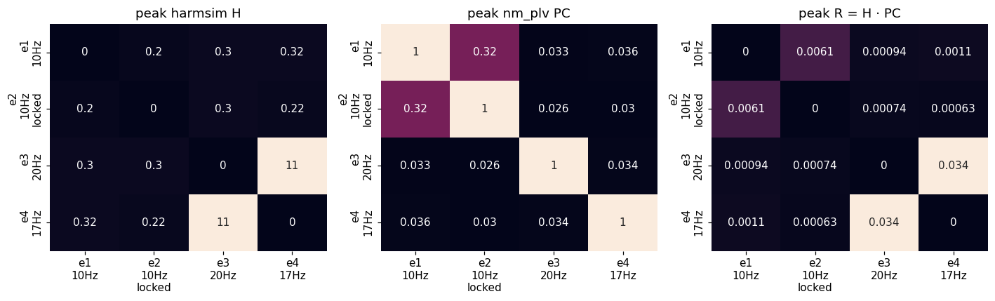
10a. Peak-based connectivity (legacy + new)

# Legacy peak-based H: harmsim
M_harmsim = hc.compute_harm_connectivity(metric='harmsim', graph=False)

# New: peak-based phase coupling (registry-dispatched)
M_pc = hc.compute_peak_phase_coupling_connectivity(
    coupling_metric='nm_plv', graph=False,
)

# New: peak-based H × PC = R
M_r = hc.compute_peak_resonance_connectivity(
    harm_metric='harmsim', coupling_metric='nm_plv', combine='product',
    graph=False,
)

import seaborn as sns
labels = ['e1\n10Hz', 'e2\n10Hz\nlocked', 'e3\n20Hz', 'e4\n17Hz']
fig, axes = plt.subplots(1, 3, figsize=(13, 4))
for ax, M, title in zip(axes, [M_harmsim, M_pc, M_r],
                         ['peak harmsim H', 'peak nm_plv PC', 'peak R = H · PC']):
    sns.heatmap(np.nan_to_num(M), ax=ax, annot=True, fmt='.2g',
                xticklabels=labels, yticklabels=labels, cbar=False)
    ax.set_title(title)
plt.tight_layout(); plt.show()

C:\Users\skite\miniconda3\envs\py310\lib\site-packages\numpy\core\fromnumeric.py:3504: RuntimeWarning: Mean of empty slice.
  return _methods._mean(a, axis=axis, dtype=dtype,
C:\Users\skite\miniconda3\envs\py310\lib\site-packages\numpy\core\_methods.py:129: RuntimeWarning: invalid value encountered in scalar divide
  ret = ret.dtype.type(ret / rcount)
C:\Users\skite\miniconda3\envs\py310\lib\site-packages\numpy\core\fromnumeric.py:3504: RuntimeWarning: Mean of empty slice.
  return _methods._mean(a, axis=axis, dtype=dtype,
C:\Users\skite\miniconda3\envs\py310\lib\site-packages\numpy\core\_methods.py:129: RuntimeWarning: invalid value encountered in scalar divide
  ret = ret.dtype.type(ret / rcount)
C:\Users\skite\miniconda3\envs\py310\lib\site-packages\numpy\core\fromnumeric.py:3504: RuntimeWarning: Mean of empty slice.
  return _methods._mean(a, axis=axis, dtype=dtype,
C:\Users\skite\miniconda3\envs\py310\lib\site-packages\numpy\core\_methods.py:129: RuntimeWarning: invalid value encountered in scalar divide
  ret = ret.dtype.type(ret / rcount)
C:\Users\skite\miniconda3\envs\py310\lib\site-packages\numpy\core\fromnumeric.py:3504: RuntimeWarning: Mean of empty slice.
  return _methods._mean(a, axis=axis, dtype=dtype,
C:\Users\skite\miniconda3\envs\py310\lib\site-packages\numpy\core\_methods.py:129: RuntimeWarning: invalid value encountered in scalar divide
  ret = ret.dtype.type(ret / rcount)

C:\Users\skite\miniconda3\envs\py310\lib\site-packages\numpy\core\fromnumeric.py:3504: RuntimeWarning: Mean of empty slice.
  return _methods._mean(a, axis=axis, dtype=dtype,
C:\Users\skite\miniconda3\envs\py310\lib\site-packages\numpy\core\_methods.py:129: RuntimeWarning: invalid value encountered in scalar divide
  ret = ret.dtype.type(ret / rcount)
C:\Users\skite\miniconda3\envs\py310\lib\site-packages\numpy\core\fromnumeric.py:3504: RuntimeWarning: Mean of empty slice.
  return _methods._mean(a, axis=axis, dtype=dtype,
C:\Users\skite\miniconda3\envs\py310\lib\site-packages\numpy\core\_methods.py:129: RuntimeWarning: invalid value encountered in scalar divide
  ret = ret.dtype.type(ret / rcount)
C:\Users\skite\miniconda3\envs\py310\lib\site-packages\numpy\core\fromnumeric.py:3504: RuntimeWarning: Mean of empty slice.
  return _methods._mean(a, axis=axis, dtype=dtype,
C:\Users\skite\miniconda3\envs\py310\lib\site-packages\numpy\core\_methods.py:129: RuntimeWarning: invalid value encountered in scalar divide
  ret = ret.dtype.type(ret / rcount)
C:\Users\skite\miniconda3\envs\py310\lib\site-packages\numpy\core\fromnumeric.py:3504: RuntimeWarning: Mean of empty slice.
  return _methods._mean(a, axis=axis, dtype=dtype,
C:\Users\skite\miniconda3\envs\py310\lib\site-packages\numpy\core\_methods.py:129: RuntimeWarning: invalid value encountered in scalar divide
  ret = ret.dtype.type(ret / rcount)

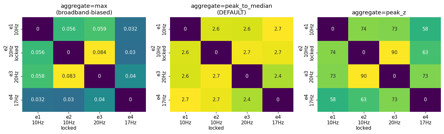
10b. Spectrum-based cross-resonance matrix

# Spectrum-based: loop compute_cross_resonance over all pairs
cfg = ResonanceConfig(precision_hz=0.5, fmin=2, fmax=30)

M_max = hc.compute_cross_resonance_connectivity(
    config=cfg, factor='R', flavor='all', aggregate='max', graph=False,
)
M_p2m = hc.compute_cross_resonance_connectivity(
    config=cfg, factor='R', flavor='all', aggregate='peak_to_median', graph=False,
)
M_pz = hc.compute_cross_resonance_connectivity(
    config=cfg, factor='R', flavor='all', aggregate='peak_z', graph=False,
)

fig, axes = plt.subplots(1, 3, figsize=(13, 4))
for ax, M, title in zip(axes, [M_max, M_p2m, M_pz],
                         ['aggregate=max\n(broadband-biased)',
                          'aggregate=peak_to_median\n(DEFAULT)',
                          'aggregate=peak_z']):
    sns.heatmap(np.nan_to_num(M), ax=ax, annot=True, fmt='.2g',
                xticklabels=labels, yticklabels=labels, cbar=False,
                cmap='viridis')
    ax.set_title(title)
plt.tight_layout(); plt.show()

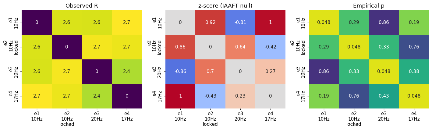
10c. Statistical inference: surrogate-z-scored connectivity matrix

For paper-quality discrimination between true cross-channel phase coupling and broadband-power artifacts, run the connectivity matrix against an IAAFT surrogate null (preserves per-channel PSD, destroys cross-channel phase). High z-scores = real coupling above the broadband baseline.

obs, z_matrix, p_matrix = hc.compute_cross_resonance_connectivity_zscore(
    config=cfg, factor='R', flavor='all', aggregate='peak_to_median',
    surrogate_kind='iaaft', n_surrogates=20, rng_seed=42,
    graph=False,
)

fig, axes = plt.subplots(1, 3, figsize=(13, 4))
for ax, M, title, cmap, kw in [
    (axes[0], obs, "Observed R", "viridis", {}),
    (axes[1], z_matrix, "z-score (IAAFT null)", "coolwarm", {"center": 0}),
    (axes[2], p_matrix, "Empirical p", "viridis_r", {"vmin": 0, "vmax": 1}),
]:
    sns.heatmap(np.nan_to_num(M), ax=ax, annot=True, fmt='.2g',
                xticklabels=labels, yticklabels=labels, cbar=False,
                cmap=cmap, **kw)
    ax.set_title(title)
plt.tight_layout(); plt.show()

C:\Users\skite\Documents\Github\biotuner\.claude\worktrees\sweet-hamilton-6c0f0d\biotuner\harmonic_connectivity.py:949: RuntimeWarning: Mean of empty slice
  mu = np.nanmean(surr_stack, axis=0)
C:\Users\skite\miniconda3\envs\py310\lib\site-packages\numpy\lib\nanfunctions.py:1879: RuntimeWarning: Degrees of freedom <= 0 for slice.
  var = nanvar(a, axis=axis, dtype=dtype, out=out, ddof=ddof,

11. Reproducing legacy compute_global_harmonicity

Existing analyses that used the pre-refactor compute_global_harmonicity reproduce bit-exactly by passing the legacy preset ResonanceConfig.

# Build a legacy-equivalent ResonanceConfig
legacy_cfg = ResonanceConfig(
    psd_normalization='minmax_prob',           # legacy two-step PSD norm
    harmonic_kernel='harmsim',
    harmonic_kernel_params={'n_harms': 10, 'delta_lim': 20, 'min_notes': 2},
    ratio_kernel='binary',
    ratio_kernel_params={'max_nm': 3, 'tolerance': 0.05, 'fallback_to_1_1': True},
    phase_estimator='stft',
    coupling_metric='nm_plv',                  # legacy convention
    gaussian_smooth_sigma=1.0,
    legacy_self_pair_subtract=True,
    normalize=True, bandwidth_correction=False,
    combine='product',
)

sig = harmonic_signal()
result_legacy = compute_resonance(sig, sf=SF, config=legacy_cfg)
print("This reproduces the pre-refactor compute_global_harmonicity numerics "
      "within float-precision.")
print("Recommended for: reproducing published paper outputs only.")

This reproduces the pre-refactor compute_global_harmonicity numerics within float-precision.
Recommended for: reproducing published paper outputs only.

For new analyses, the recommended config is the default:

result = compute_resonance(signal, sf=1000)

which uses the refined defaults (joint PC reducer, n:m ratio kernel where applicable, nm_plv_canonical-compatible conventions).

---

Further reading

• Module docstrings — help(biotuner.resonance), help(biotuner.harmonic_spectrum), help(biotuner.harmonic_connectivity) — each has a Quick Start.

• list_strategies() — discoverable inventory of every registered kernel, metric, and combine rule.

• Sphinx API docs — under docs/api/resonance.rst, docs/api/harmonic_spectrum.rst, docs/api/harmonic_connectivity.rst.

• Plan — biotuner_resonance_plan.md documents the full Phase 1 / 2 / 3 roadmap and references for every algorithm.

What’s not in this notebook (Phase 2/3 additions)

The registry slots exist for these but aren’t filled yet:

• More harmonic kernels: sethares, stolzenburg, hopf, lorentzian, harmonic_entropy, plus the existing-but-not-wired biotuner metrics tenney_height, euler, compute_consonance, integral_tenney_height.

• More ratio kernels: arnold_tongue (soft Gaussian), stern_brocot.

• More phase estimators: hilbert_bandpass, morlet_wavelet.

• Higher-order coupling: bplv (triplet), mplv (N-ary), cf_plm, gpla.

• Persistence (Q-factor) axis: lagged_coherence, lhac, fooof_bandwidth.

Each lands as a one-line register_* call against the existing registry — contributions welcome.