Plotting and visualization with biotuner

This notebook walks through the biotuner plotting API on rich synthetic signals that produce well-populated, “garnished” figures. We cover single-series peak analysis, tuning visualization, harmonic-fit diagnostics, multi-channel dissonance curves, and group-level plots on a BiotunerGroup.

Table of contents

1. Setup and synthetic signals

2. Peak analysis plots

3. Tuning visualization

4. Harmonic-fit diagnostics

5. Multi-channel dissonance curve

6. Group analysis plots (BiotunerGroup)

7. 3D group heatmaps (trials × channels)

1. Setup and synthetic signals

We build three synthetic signals chosen to highlight different aspects of the plotting API:

• Signal A — harmonic stack. A clean fundamental at 5 Hz with octave and inner harmonics (5, 10, 15, 20, 25, 30, 40 Hz). Yields tight ratios and rich dissonance curves.

• Signal B — just-intonation chord. A 4:5:6:7:8:10 chord centered around 6 Hz. Highlights septimal intervals.

• Signal C — EEG-like multi-band. Theta + alpha + beta + gamma with realistic noise. Produces a busier spectrum and broader peak distribution.

import numpy as np
import matplotlib.pyplot as plt

from biotuner.biotuner_object import compute_biotuner
from biotuner.biotuner_group import BiotunerGroup
from biotuner.plot_config import set_biotuner_style
from biotuner.vizs import diss_curve_multi

set_biotuner_style()

rng = np.random.default_rng(7)
sf = 1000
duration = 8
t = np.linspace(0, duration, sf * duration, endpoint=False)


def make_signal(freqs, amps, noise=0.05):
    sig = sum(a * np.sin(2 * np.pi * f * t) for f, a in zip(freqs, amps))
    return sig + noise * rng.standard_normal(len(t))


# A — dense harmonic stack
sig_A = make_signal(
    [5, 10, 15, 20, 25, 30, 40],
    [1.0, 0.8, 0.6, 0.5, 0.4, 0.3, 0.2],
    noise=0.05,
)

# B — just-intonation chord (4:5:6:7:8:10) on a 6 Hz base
base = 6
sig_B = make_signal(
    [base * r for r in (1, 5/4, 6/4, 7/4, 8/4, 10/4)],
    [1.0, 0.85, 0.75, 0.6, 0.5, 0.4],
    noise=0.06,
)

# C — EEG-like
sig_C = make_signal(
    [6, 10, 12, 22, 30, 45],
    [0.8, 1.0, 0.7, 0.5, 0.4, 0.3],
    noise=0.25,
)

print(f"sig_A: {sig_A.shape}, sig_B: {sig_B.shape}, sig_C: {sig_C.shape}")

sig_A: (8000,), sig_B: (8000,), sig_C: (8000,)

We instantiate three compute_biotuner objects, extract peaks, compute metrics, and pre-compute the dissonance and harmonic-entropy curves so every downstream plot has its data ready.

def build_bt(signal, label, peaks_function="harmonic_recurrence",
             min_freq=2, max_freq=50, n_peaks=7):
    bt = compute_biotuner(
        sf=sf,
        peaks_function=peaks_function,
        precision=0.25,
        n_harm=10,
    )
    bt.peaks_extraction(
        signal,
        min_freq=min_freq,
        max_freq=max_freq,
        n_peaks=n_peaks,
        min_harms=2,
        ratios_extension=True,
        graph=False,
    )
    bt.compute_peaks_metrics()
    # extend peaks so the dissonance curve is densely populated
    bt.peaks_extension(method="harmonic_fit", n_harm=10,
                       cons_limit=0.1, ratios_extension=False)
    bt.compute_diss_curve(input_type="extended_peaks",
                          denom=100, max_ratio=2,)
    print(f"{label:>22s}  peaks = {np.round(bt.peaks, 2)}")
    return bt


bt_A = build_bt(sig_A, "A — harmonic stack")
bt_B = build_bt(sig_B, "B — JI chord")
bt_C = build_bt(sig_C, "C — EEG-like")

    A — harmonic stack  peaks = [ 2.5   5.    3.   10.   15.    8.25 20.  ]
          B — JI chord  peaks = [ 3.75  2.75  7.5   6.    9.   10.5  16.5 ]
          C — EEG-like  peaks = [ 3.5   6.   12.   10.   30.   18.25 15.  ]

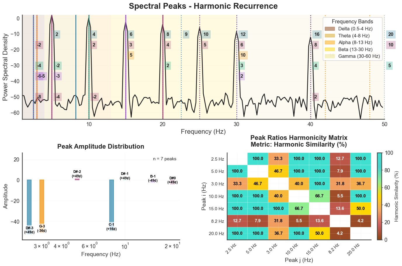
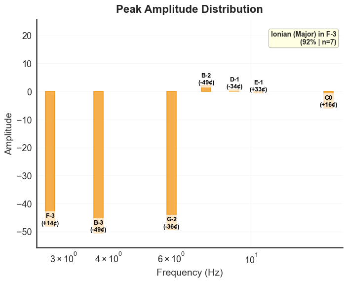
2. Peak analysis plots

plot_peaks(show_matrix=True) returns a 3-panel figure: power-spectrum with peak markers, peak amplitudes (with note labels), and the peak harmonicity matrix. This is the most informative single view of a biotuner object.

bt_A.plot_peaks(xmin=1, xmax=50, show_matrix=True)
plt.show()

C:\Users\skite\Documents\Github\biotuner\biotuner\plot_utils.py:1138: UserWarning: This figure includes Axes that are not compatible with tight_layout, so results might be incorrect.
  plt.tight_layout()

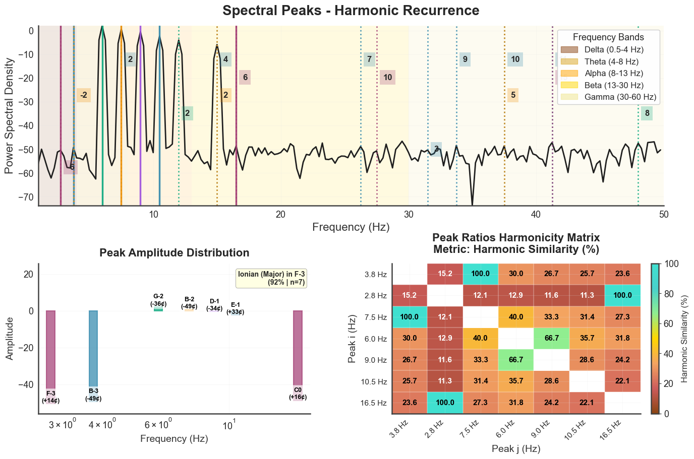
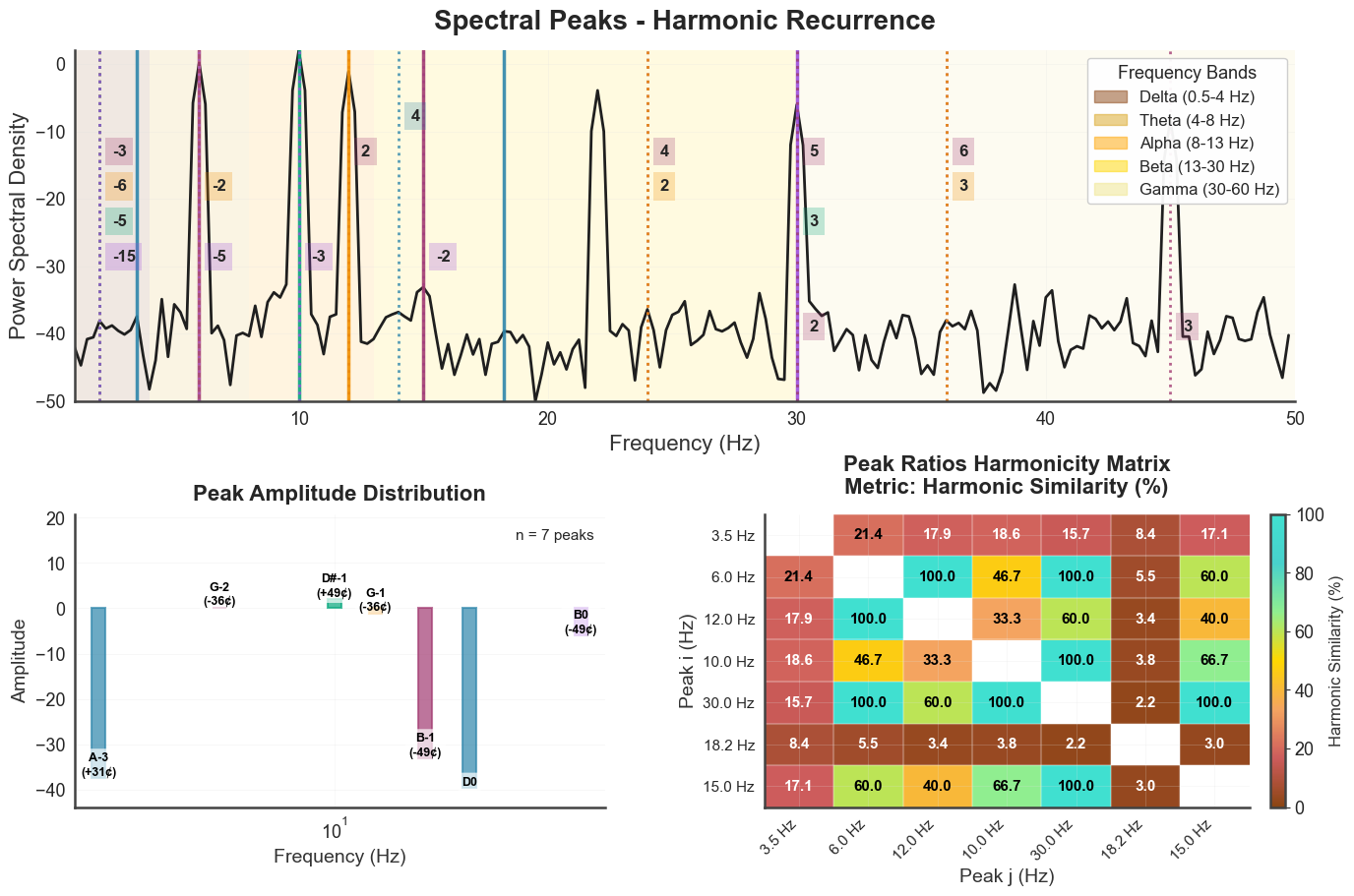
Same plot for the JI chord and the EEG-like signal:

bt_B.plot_peaks(xmin=1, xmax=50, show_matrix=True)
plt.show()

C:\Users\skite\Documents\Github\biotuner\biotuner\plot_utils.py:1138: UserWarning: This figure includes Axes that are not compatible with tight_layout, so results might be incorrect.
  plt.tight_layout()

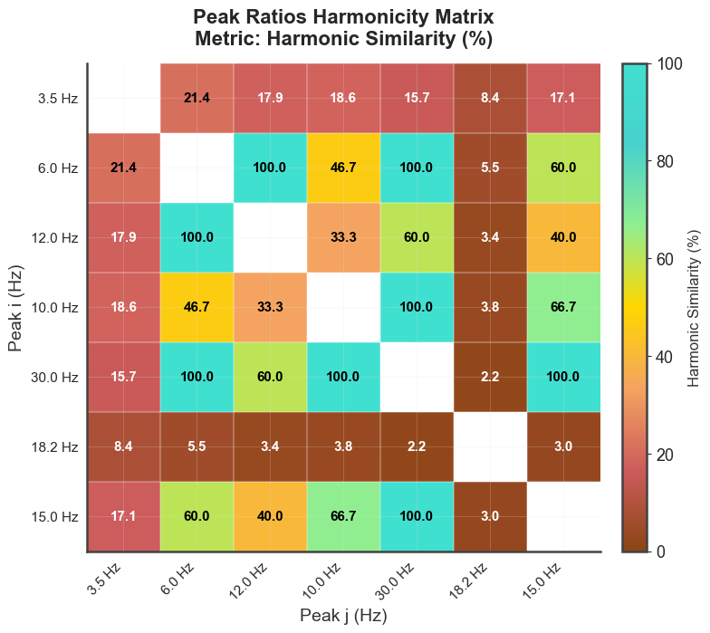
bt_C.plot_peaks(xmin=1, xmax=50, show_matrix=True)
plt.show()

C:\Users\skite\Documents\Github\biotuner\biotuner\plot_utils.py:1138: UserWarning: This figure includes Axes that are not compatible with tight_layout, so results might be incorrect.
  plt.tight_layout()

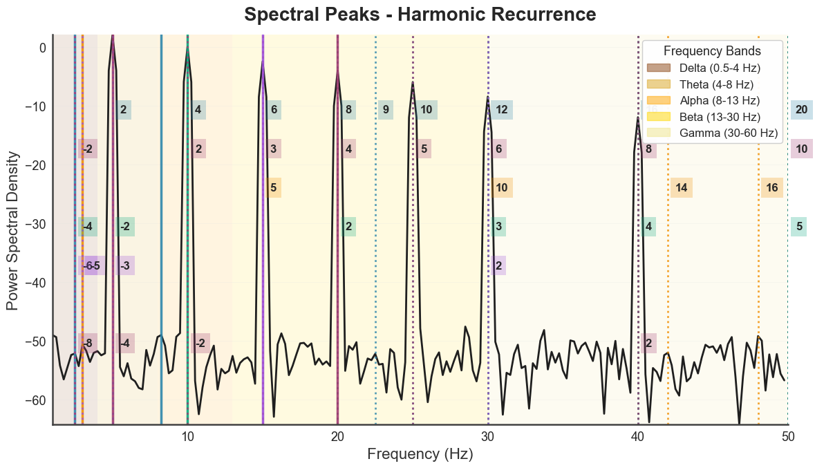
The individual panels are also exposed as standalone methods, useful for embedding a single panel in a custom layout.

# spectrum-only view
bt_A.plot_peaks_spectrum(xmin=1, xmax=50)
plt.show()

# amplitude bars with musical-note labels
bt_B.plot_peaks_amplitude(xmin=1, xmax=50)
plt.show()

# harmonicity matrix between peak pairs
bt_C.plot_peaks_matrix(metric="harmsim")
plt.show()

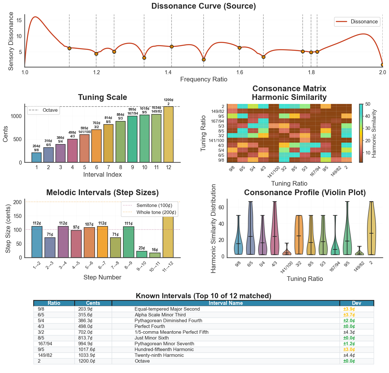
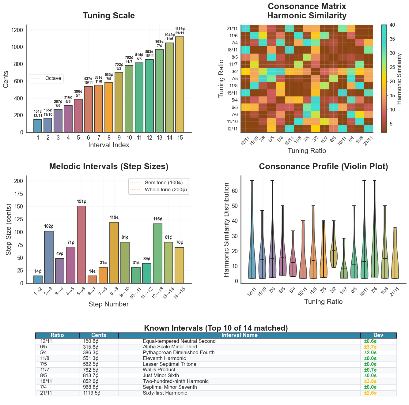
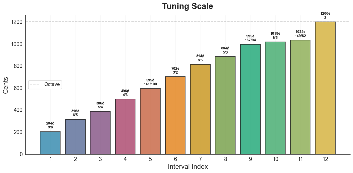
3. Tuning visualization

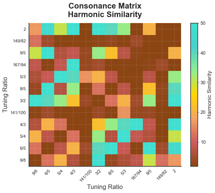
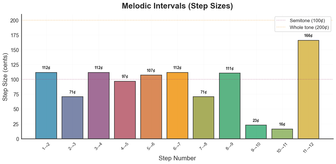
plot_tuning() is the workhorse for scale visualization. With panels=4, show_source_curve=True it produces a four-panel summary: source curve at the top, then scale steps, consonance matrix, and step-size intervals. The tuning argument selects which scale to display (peaks_ratios, diss_curve, harm_tuning, harm_fit_tuning, euler_fokker, HE).

bt_A.plot_tuning(tuning="diss_curve", metric="harmsim",
                 panels=4, show_source_curve=True)
plt.show()

C:\Users\skite\Documents\Github\biotuner\biotuner\plot_utils.py:2348: UserWarning: This figure includes Axes that are not compatible with tight_layout, so results might be incorrect.
  plt.tight_layout()
C:\Users\skite\Documents\Github\biotuner\biotuner\plot_utils.py:2497: UserWarning: This figure includes Axes that are not compatible with tight_layout, so results might be incorrect.
  plt.tight_layout()
C:\Users\skite\Documents\Github\biotuner\biotuner\plot_utils.py:2571: UserWarning: This figure includes Axes that are not compatible with tight_layout, so results might be incorrect.
  plt.tight_layout()
C:\Users\skite\Documents\Github\biotuner\biotuner\plot_utils.py:2724: UserWarning: This figure includes Axes that are not compatible with tight_layout, so results might be incorrect.
  plt.tight_layout()

bt_B.plot_tuning(tuning="peaks_ratios", metric="harmsim",
                 panels=4, show_source_curve=True)
plt.show()

C:\Users\skite\Documents\Github\biotuner\biotuner\plot_utils.py:2348: UserWarning: This figure includes Axes that are not compatible with tight_layout, so results might be incorrect.
  plt.tight_layout()
C:\Users\skite\Documents\Github\biotuner\biotuner\plot_utils.py:2497: UserWarning: This figure includes Axes that are not compatible with tight_layout, so results might be incorrect.
  plt.tight_layout()
C:\Users\skite\Documents\Github\biotuner\biotuner\plot_utils.py:2571: UserWarning: This figure includes Axes that are not compatible with tight_layout, so results might be incorrect.
  plt.tight_layout()
C:\Users\skite\Documents\Github\biotuner\biotuner\plot_utils.py:2724: UserWarning: This figure includes Axes that are not compatible with tight_layout, so results might be incorrect.
  plt.tight_layout()

Each panel is also available individually:

bt_A.plot_tuning_scale(tuning="diss_curve")
plt.show()

bt_A.plot_tuning_matrix(tuning="diss_curve", metric="harmsim")
plt.show()

bt_A.plot_tuning_intervals(tuning="diss_curve")
plt.show()

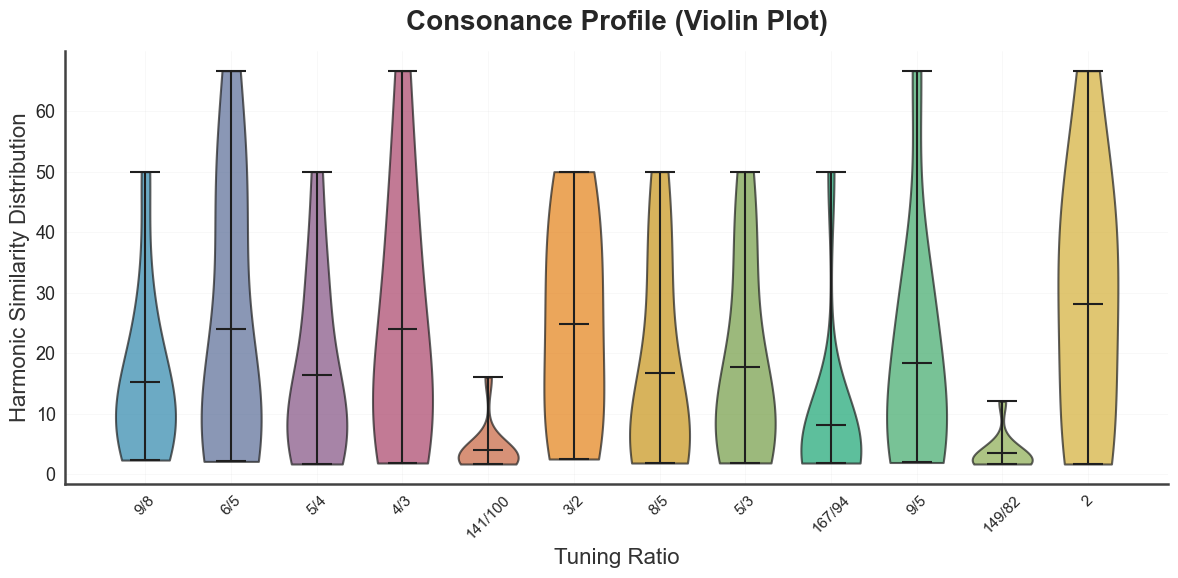
bt_A.plot_tuning_consonance_profile(tuning="diss_curve", metric="harmsim")
plt.show()

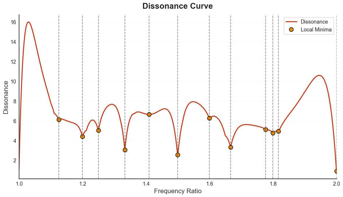
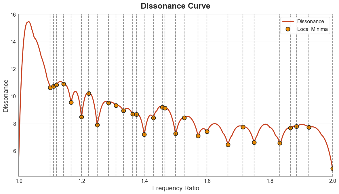
plot_tuning_curve renders the underlying source curve (dissonance or harmonic entropy) with detected minima highlighted.

bt_A.plot_tuning_curve(curve_type="dissonance")
plt.show()

bt_B.plot_tuning_curve(curve_type="dissonance")
plt.show()

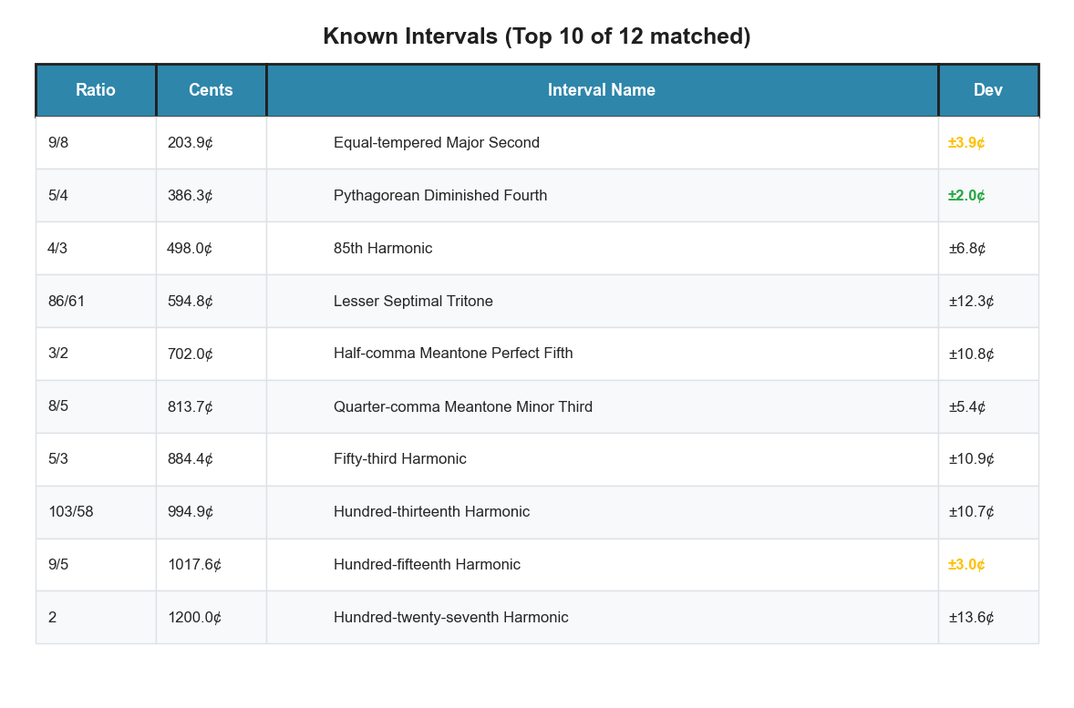
plot_tuning_interval_table annotates each scale step with the closest named just-intonation interval, within a tolerance you set.

bt_A.plot_tuning_interval_table(tuning="diss_curve",
                                max_denom=64, tolerance_cents=15)
plt.show()

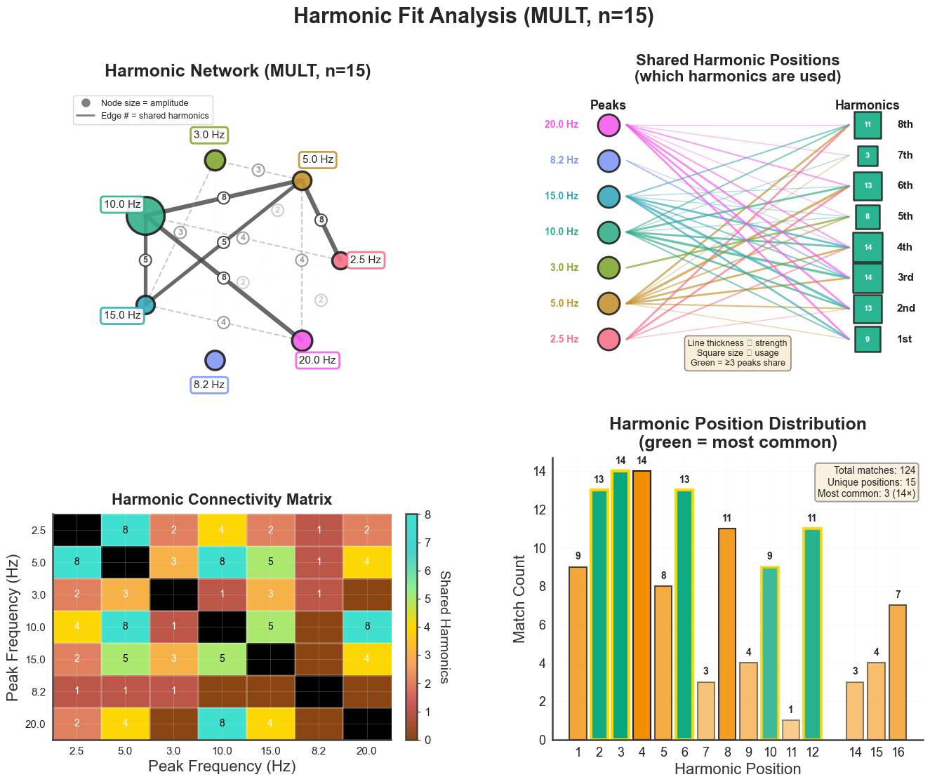
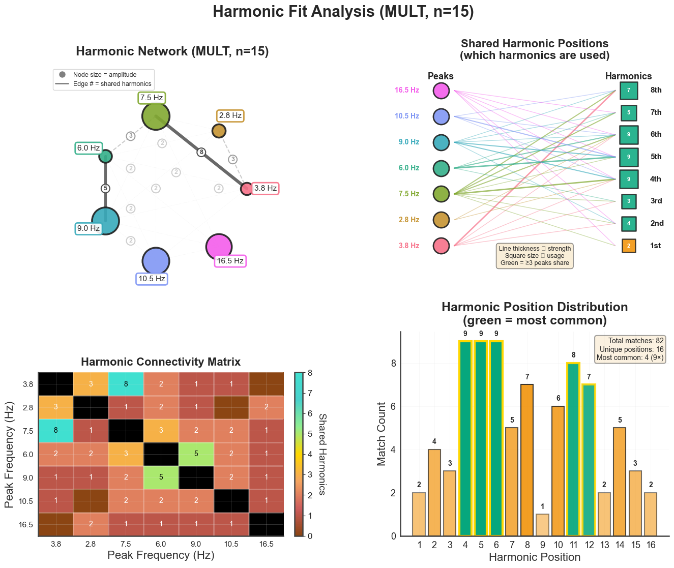
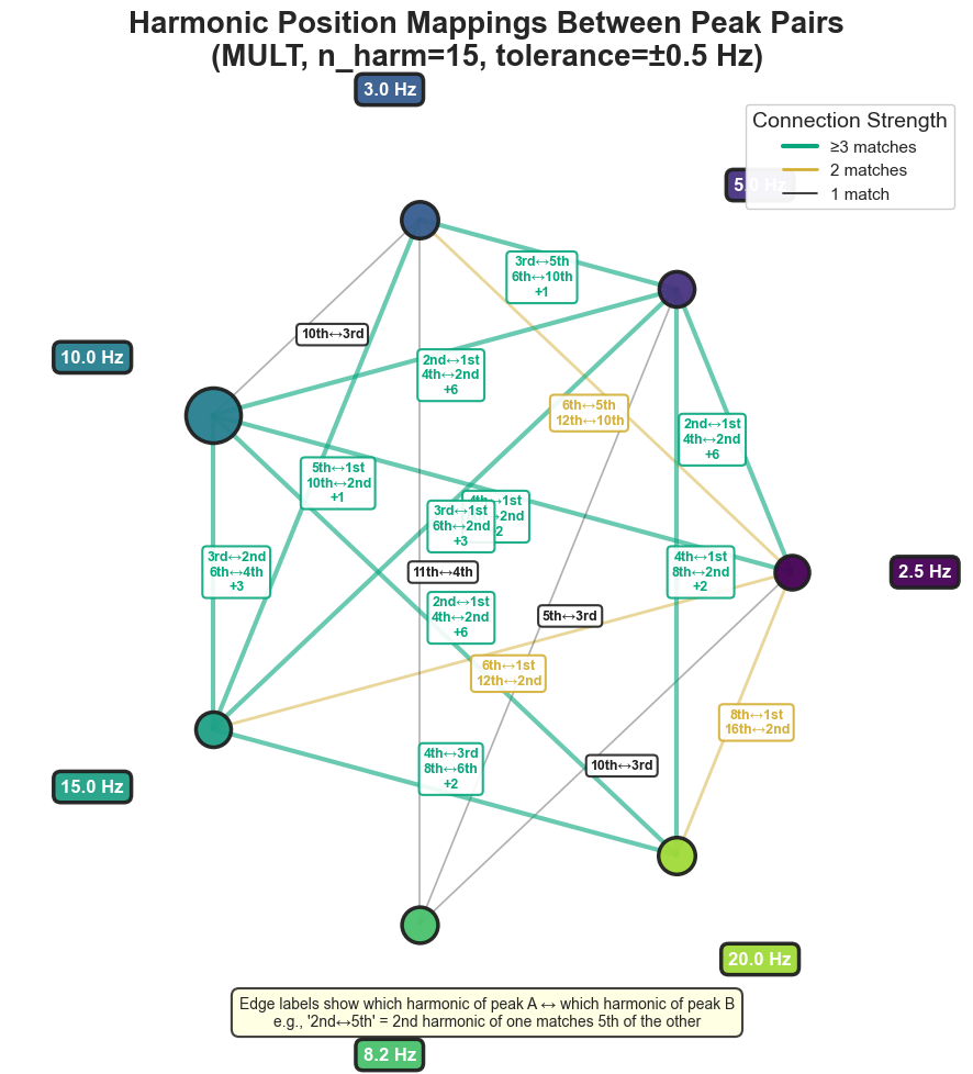
4. Harmonic-fit diagnostics

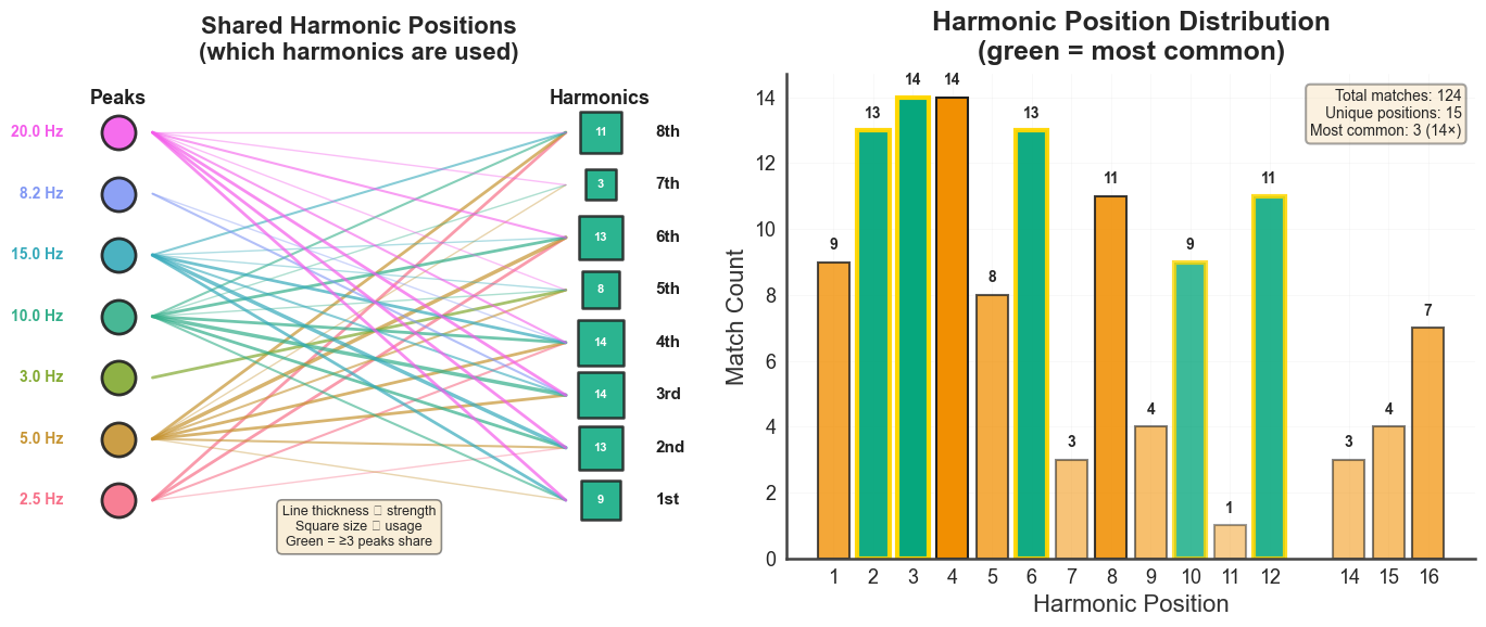
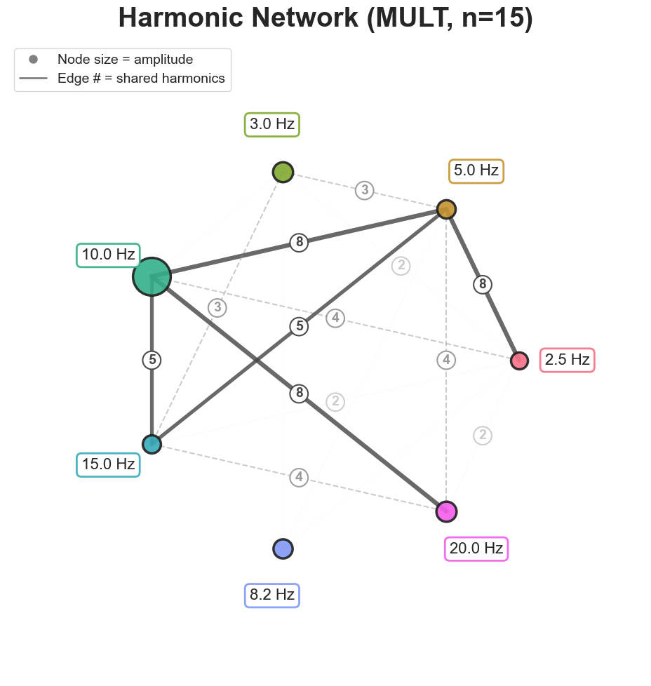
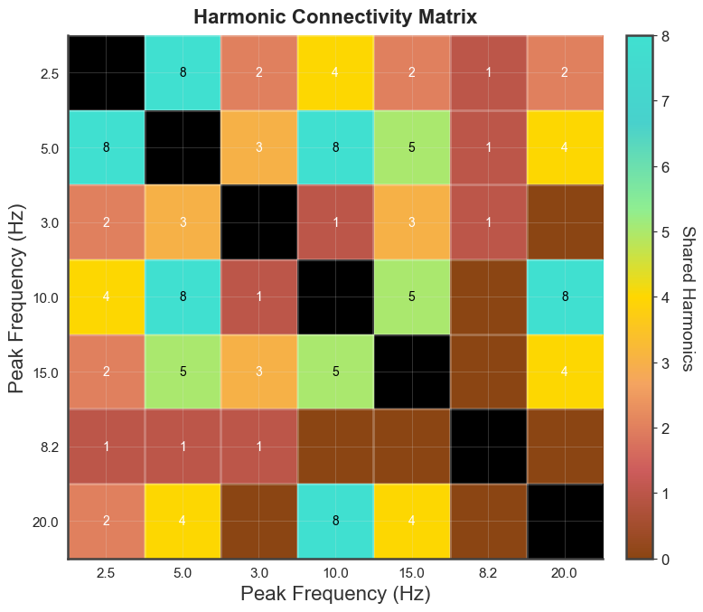
plot_harmonic_fit() produces a 2×2 panel showing how well the spectral peaks fit a shared harmonic series. Top-left: PSD with peak markers and extension positions; top-right: harmonic positions per peak; bottom-left: harmonic-fit network (which harmonic of which peak coincides with which other peak); bottom-right: connectivity matrix.

bt_A.plot_harmonic_fit(n_harm=15, harm_bounds=0.5)
plt.show()

C:\Users\skite\Documents\Github\biotuner\biotuner\plot_utils.py:3884: UserWarning: This figure includes Axes that are not compatible with tight_layout, so results might be incorrect.
  plt.tight_layout()
C:\Users\skite\Documents\Github\biotuner\biotuner\plot_utils.py:3990: UserWarning: This figure includes Axes that are not compatible with tight_layout, so results might be incorrect.
  plt.tight_layout()
C:\Users\skite\Documents\Github\biotuner\biotuner\plot_utils.py:4221: UserWarning: This figure includes Axes that are not compatible with tight_layout, so results might be incorrect.
  plt.tight_layout()
C:\Users\skite\Documents\Github\biotuner\biotuner\plot_utils.py:4366: UserWarning: This figure includes Axes that are not compatible with tight_layout, so results might be incorrect.
  plt.tight_layout(rect=[0, 0, 1, 0.96])
c:\Users\skite\miniconda3\envs\biotuner_env\Lib\site-packages\IPython\core\pylabtools.py:170: UserWarning: Glyph 8733 (\N{PROPORTIONAL TO}) missing from font(s) Arial.
  fig.canvas.print_figure(bytes_io, **kw)

bt_B.plot_harmonic_fit(n_harm=15, harm_bounds=0.5)
plt.show()

C:\Users\skite\Documents\Github\biotuner\biotuner\plot_utils.py:3884: UserWarning: This figure includes Axes that are not compatible with tight_layout, so results might be incorrect.
  plt.tight_layout()
C:\Users\skite\Documents\Github\biotuner\biotuner\plot_utils.py:3990: UserWarning: This figure includes Axes that are not compatible with tight_layout, so results might be incorrect.
  plt.tight_layout()
C:\Users\skite\Documents\Github\biotuner\biotuner\plot_utils.py:4221: UserWarning: This figure includes Axes that are not compatible with tight_layout, so results might be incorrect.
  plt.tight_layout()
C:\Users\skite\Documents\Github\biotuner\biotuner\plot_utils.py:4366: UserWarning: This figure includes Axes that are not compatible with tight_layout, so results might be incorrect.
  plt.tight_layout(rect=[0, 0, 1, 0.96])
c:\Users\skite\miniconda3\envs\biotuner_env\Lib\site-packages\IPython\core\pylabtools.py:170: UserWarning: Glyph 8733 (\N{PROPORTIONAL TO}) missing from font(s) Arial.
  fig.canvas.print_figure(bytes_io, **kw)

Each subview is exposed as its own method:

bt_A.plot_harmonic_fit_network(n_harm=15, harm_bounds=0.5)
plt.show()

bt_A.plot_harmonic_fit_matrix(n_harm=15, harm_bounds=0.5)
plt.show()

bt_A.plot_harmonic_fit_positions(n_harm=15, harm_bounds=0.5)
plt.show()

bt_A.plot_harmonic_position_mappings(n_harm=15)
plt.show()

C:\Users\skite\Documents\Github\biotuner\biotuner\plot_utils.py:4221: UserWarning: Glyph 8733 (\N{PROPORTIONAL TO}) missing from font(s) Arial.
  plt.tight_layout()
c:\Users\skite\miniconda3\envs\biotuner_env\Lib\site-packages\IPython\core\pylabtools.py:170: UserWarning: Glyph 8733 (\N{PROPORTIONAL TO}) missing from font(s) Arial.
  fig.canvas.print_figure(bytes_io, **kw)

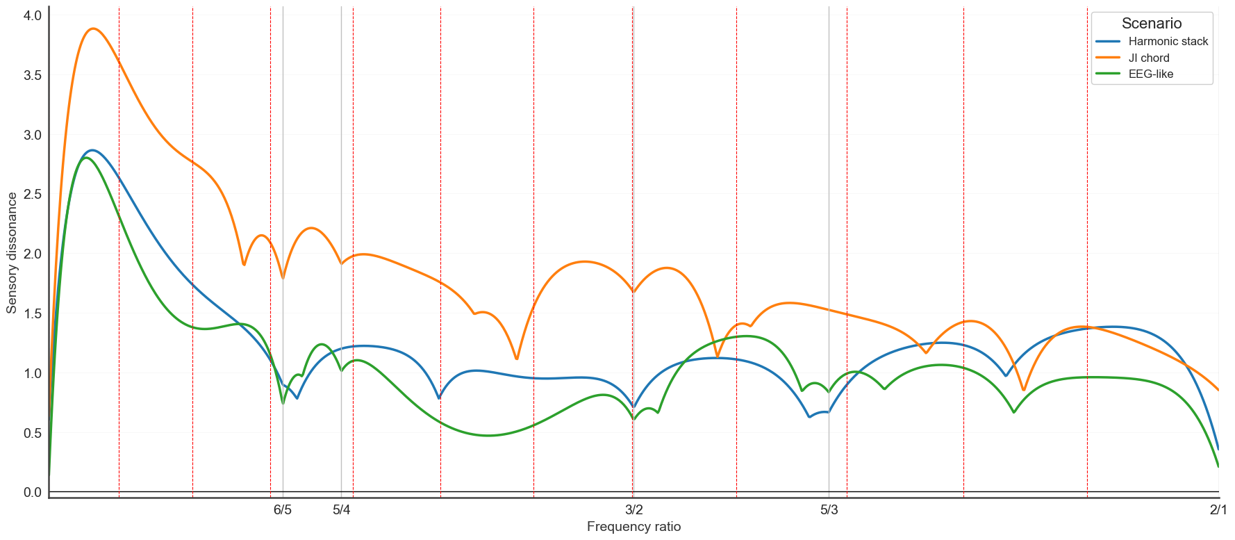
5. Multi-channel dissonance curve

diss_curve_multi overlays dissonance curves from multiple sources on a single axis and marks shared minima — useful when looking for tunings that are consistent across channels or trials.

freqs_list = [bt_A.peaks, bt_B.peaks, bt_C.peaks]
amps_list  = [bt_A.amps,  bt_B.amps,  bt_C.amps]
labels     = ["Harmonic stack", "JI chord", "EEG-like"]

plt.figure(figsize=(16, 7))
diss_curve_multi(
    freqs_list, amps_list,
    labels=labels,
    denom=12, max_ratio=2,
    n_tet_grid=12,
    data_type="Scenario",
)
plt.show()

<Figure size 1600x700 with 0 Axes>

6. Group analysis plots

BiotunerGroup orchestrates biotuner across many time series and exposes group-level plots. We build a 24-trial dataset split into two conditions (harmonic vs inharmonic) so condition-aware plots have something to compare.

N = 12
harmonic_trials = np.array([
    make_signal(
        [5 + rng.uniform(-0.2, 0.2),
         10 + rng.uniform(-0.3, 0.3),
         15 + rng.uniform(-0.3, 0.3),
         20 + rng.uniform(-0.4, 0.4),
         30 + rng.uniform(-0.5, 0.5)],
        [1.0, 0.8, 0.6, 0.5, 0.3], noise=0.1,
    ) for _ in range(N)
])
inharmonic_trials = np.array([
    make_signal(
        [4 + rng.uniform(0, 1.0),
         9 + rng.uniform(0, 1.5),
         13 + rng.uniform(0, 2.0),
         19 + rng.uniform(0, 2.0),
         27 + rng.uniform(0, 2.5)],
        [1.0, 0.7, 0.5, 0.4, 0.3], noise=0.15,
    ) for _ in range(N)
])

group_data = np.vstack([harmonic_trials, inharmonic_trials])  # (24, 8000)
metadata = {"condition": ["harmonic"] * N + ["inharmonic"] * N}
print(f"Group data: {group_data.shape}")

Group data: (24, 8000)

btg = BiotunerGroup(
    group_data, sf=sf,
    axis_labels=["trial"],
    metadata=metadata,
    peaks_function="EMD",
    precision=0.25,
)
btg.compute_peaks(min_freq=2, max_freq=50, n_peaks=6,
                  min_harms=2, verbose=False)
btg.compute_metrics()
btg.compute_diss_curve(input_type="peaks", denom=50, max_ratio=2)
summary = btg.summary()
summary.head()

Warning: 1 peaks were removed because they exceeded the maximum frequency of 50 Hz
Warning: 1 peaks were removed because they exceeded the maximum frequency of 50 Hz
Warning: 1 peaks were removed because they exceeded the maximum frequency of 50 Hz
Warning: 1 peaks were removed because they exceeded the maximum frequency of 50 Hz
Warning: 1 peaks were removed because they exceeded the maximum frequency of 50 Hz
Warning: 1 peaks were removed because they exceeded the maximum frequency of 50 Hz
Warning: 1 peaks were removed because they exceeded the maximum frequency of 50 Hz
Warning: 1 peaks were removed because they exceeded the maximum frequency of 50 Hz
Warning: 1 peaks were removed because they exceeded the maximum frequency of 50 Hz
Warning: 1 peaks were removed because they exceeded the maximum frequency of 50 Hz
Warning: 1 peaks were removed because they exceeded the maximum frequency of 50 Hz
Warning: 1 peaks were removed because they exceeded the maximum frequency of 50 Hz
Warning: 1 peaks were removed because they exceeded the maximum frequency of 50 Hz
Warning: 1 peaks were removed because they exceeded the maximum frequency of 50 Hz
Warning: 1 peaks were removed because they exceeded the maximum frequency of 50 Hz
Warning: 1 peaks were removed because they exceeded the maximum frequency of 50 Hz
Warning: 1 peaks were removed because they exceeded the maximum frequency of 50 Hz
Warning: 1 peaks were removed because they exceeded the maximum frequency of 50 Hz
Warning: 1 peaks were removed because they exceeded the maximum frequency of 50 Hz
Warning: 1 peaks were removed because they exceeded the maximum frequency of 50 Hz
Warning: 1 peaks were removed because they exceeded the maximum frequency of 50 Hz

C:\Users\skite\Documents\Github\biotuner\biotuner\metrics.py:946: RuntimeWarning: divide by zero encountered in scalar divide
  harm_temp.append(1 / delta_norm)

	trial	series_idx	condition	n_peaks	peak_freq_mean	peak_amp_mean	peak_freq_std	peak_amp_std	peak_freq_median	peak_amp_median	...	harm_pos_std	harm_pos_median	harm_pos_min	harm_pos_max	harm_pos_sem	subharm_tension	scale_dissonance	scale_diss_harm_sim	scale_diss_n_steps	common_harm_pos
0	0	0	harmonic	4	9.250000	-6.819295	6.743052	7.603799	7.625	-3.556057	...	3.136877	4.0	1.0	10.0	1.402854	0.024486	0.449587	6.318150	3	NaN
1	1	1	harmonic	4	8.062500	-8.153656	4.874599	10.155705	7.500	-3.625093	...	3.300000	5.5	1.0	11.0	1.043552	0.0	0.510659	26.809599	4	NaN
2	2	2	harmonic	4	13.500000	-10.594103	6.351673	14.275383	14.625	-3.601809	...	2.847696	4.5	1.0	10.0	1.006813	0.010381	0.784228	3.835054	3	1.0
3	3	3	harmonic	3	11.666667	-2.682947	6.371595	1.633655	9.750	-2.450868	...	1.247219	2.0	1.0	4.0	0.720082	0.025528	0.264729	4.796640	3	NaN
4	4	4	harmonic	4	13.875000	-11.281537	6.718677	12.805146	14.875	-4.127662	...	2.680951	3.0	1.0	8.0	1.340476	0.020523	0.794818	9.734093	4	NaN

5 rows × 32 columns

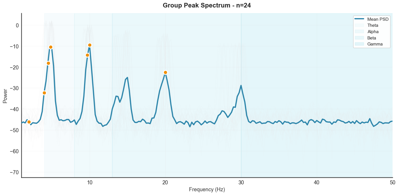
Aggregated PSD with individual traces. plot_group_peaks shows the mean spectrum across trials with per-trial overlays and detected peak markers.

btg.plot_group_peaks(show_individual=True, xmin=1, xmax=50)
plt.show()

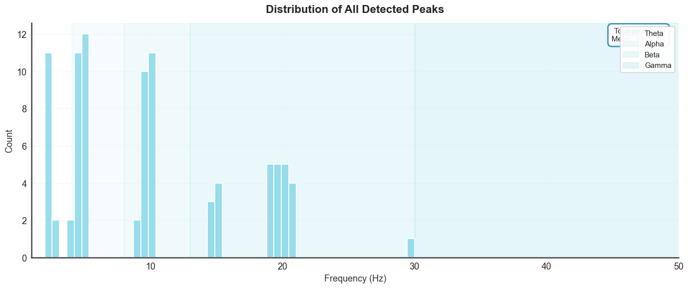
Peak frequency distribution across all trials, with band shading.

btg.plot_peak_distribution(xmin=1, xmax=50)
plt.show()

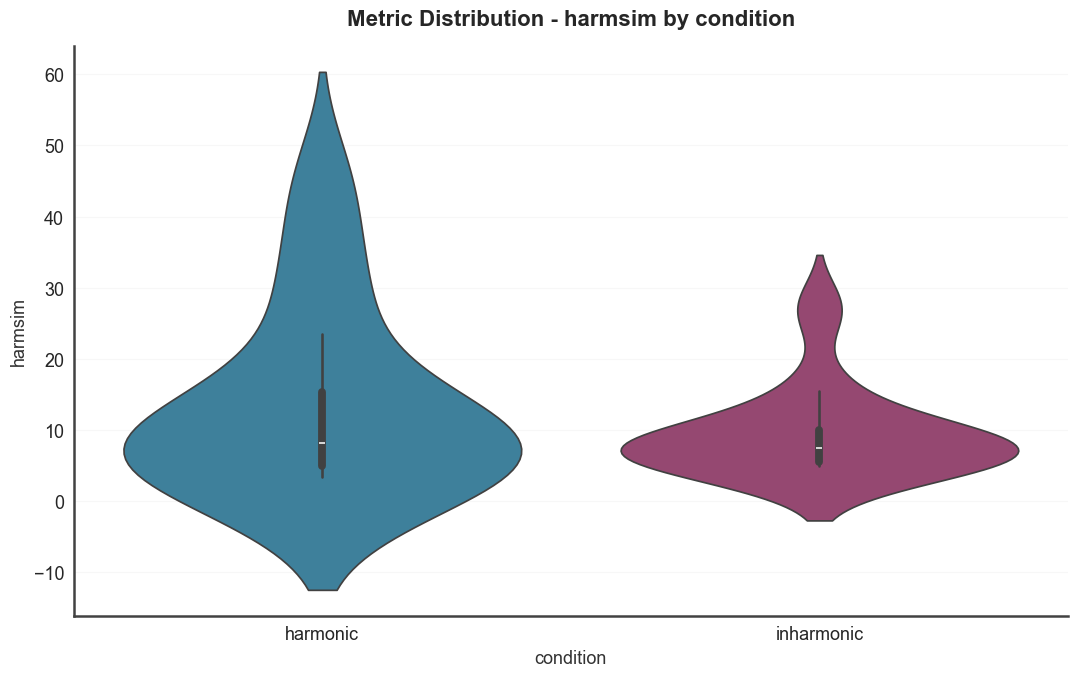
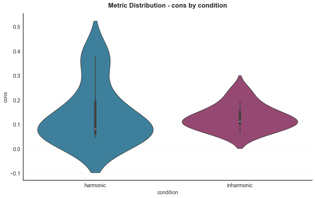
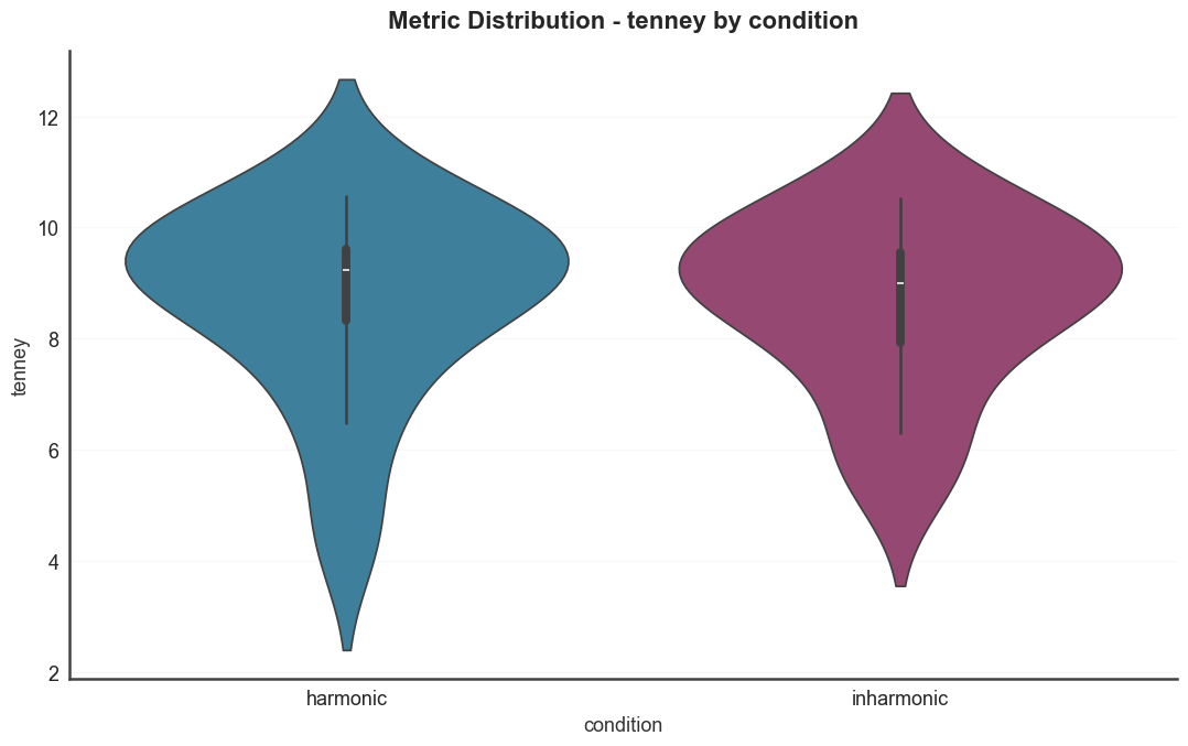
Metric distributions split by condition. Violin plots for several harmonicity metrics, colored by the condition metadata column.

for metric in ["harmsim", "cons", "tenney"]:
    btg.plot_metric_distribution(metric, groupby="condition", kind="violin")
    plt.show()

C:\Users\skite\Documents\Github\biotuner\biotuner\biotuner_group.py:1420: FutureWarning: 

Passing `palette` without assigning `hue` is deprecated and will be removed in v0.14.0. Assign the `x` variable to `hue` and set `legend=False` for the same effect.

  sns.violinplot(data=self.results, x=groupby, y=metric, ax=ax, palette=palette, **kwargs)

C:\Users\skite\Documents\Github\biotuner\biotuner\biotuner_group.py:1420: FutureWarning: 

Passing `palette` without assigning `hue` is deprecated and will be removed in v0.14.0. Assign the `x` variable to `hue` and set `legend=False` for the same effect.

  sns.violinplot(data=self.results, x=groupby, y=metric, ax=ax, palette=palette, **kwargs)

C:\Users\skite\Documents\Github\biotuner\biotuner\biotuner_group.py:1420: FutureWarning: 

Passing `palette` without assigning `hue` is deprecated and will be removed in v0.14.0. Assign the `x` variable to `hue` and set `legend=False` for the same effect.

  sns.violinplot(data=self.results, x=groupby, y=metric, ax=ax, palette=palette, **kwargs)

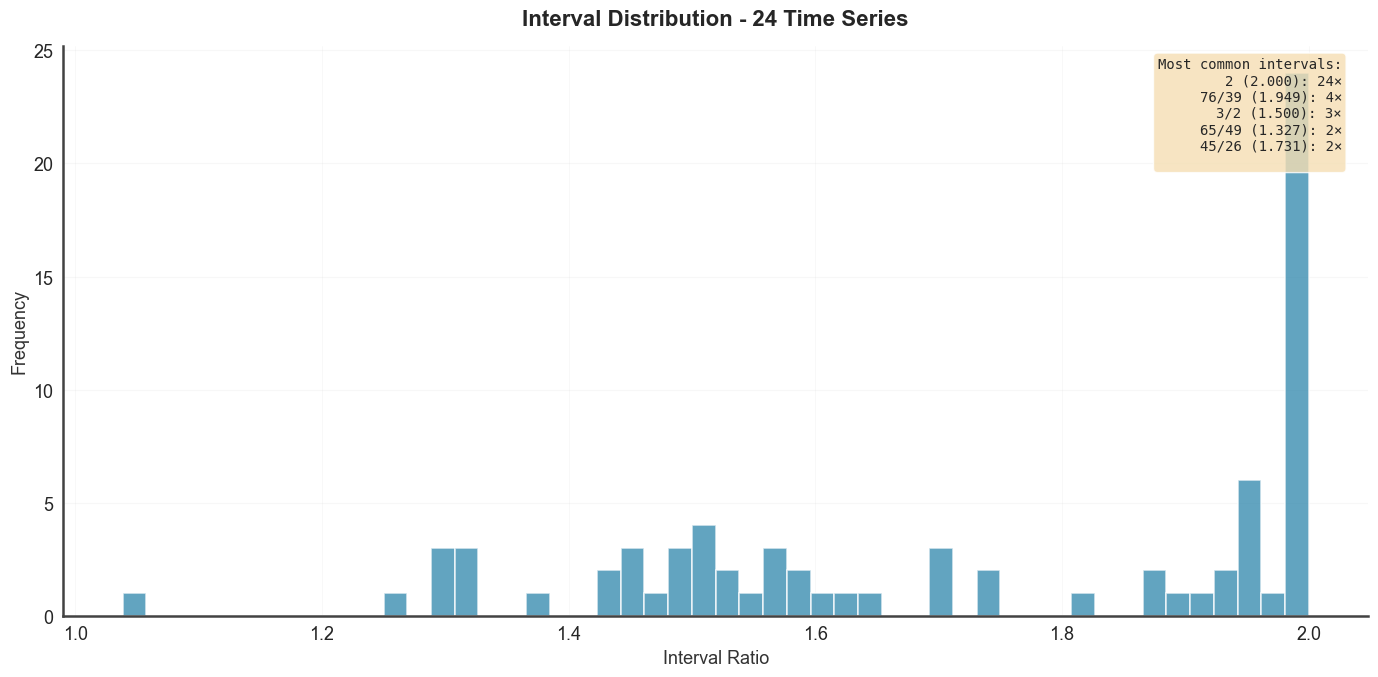
Interval histogram across all derived scales — here using the dissonance-curve scale. show_common=True overlays vertical lines at common just-intonation ratios.

btg.plot_interval_histogram("diss_scale", show_common=True, max_denom=64)
plt.show()

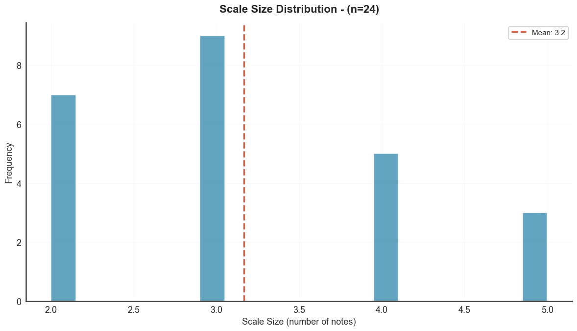
Distribution of scale sizes (number of steps per scale).

btg.plot_scale_size_distribution("diss_scale")
plt.show()

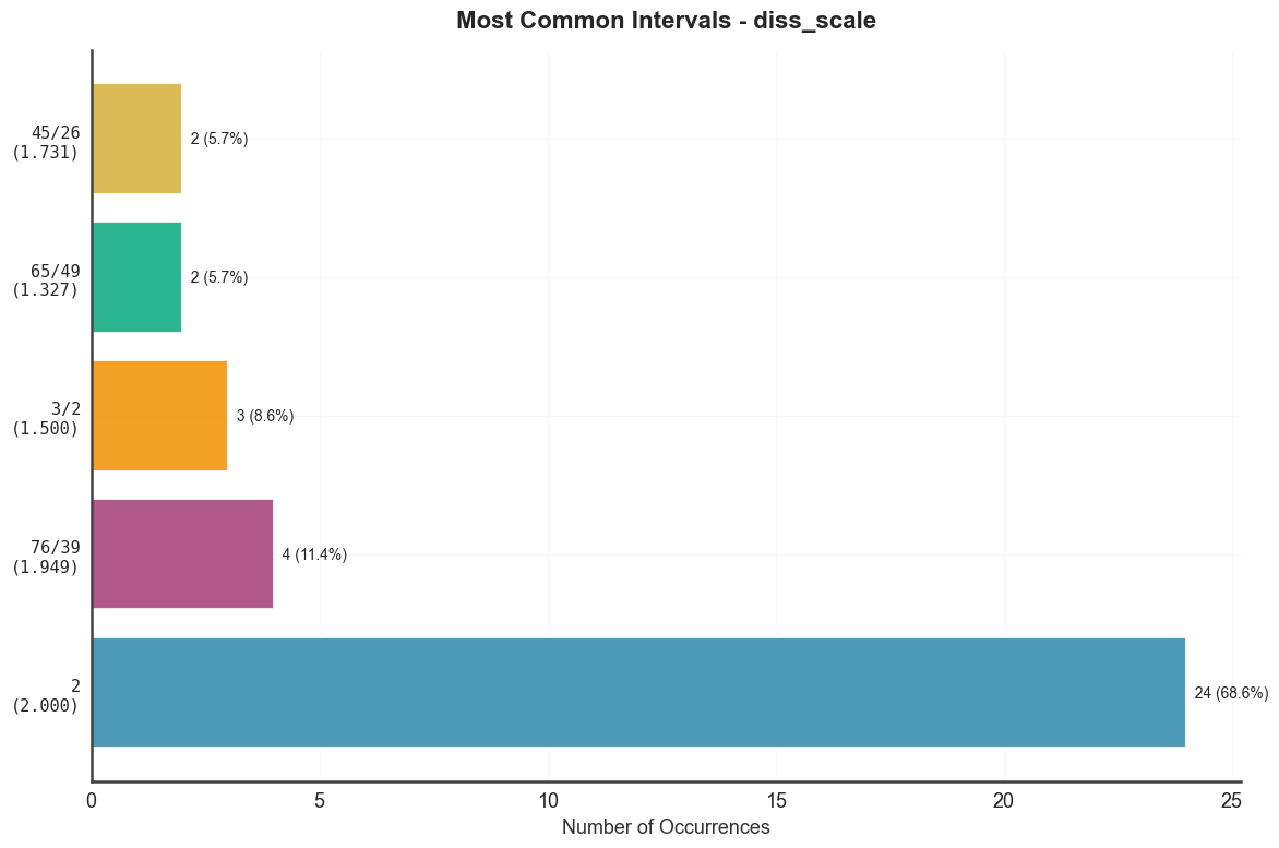
Top 15 most frequent intervals across the group.

btg.plot_common_intervals("diss_scale", top_n=15)
plt.show()

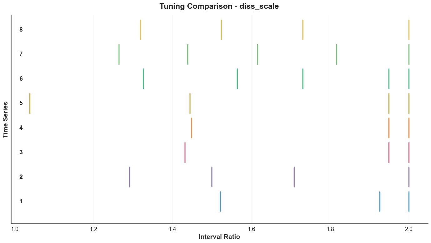
Side-by-side scale comparison for a subset of trials — each row is one trial’s tuning, with steps drawn as vertical ticks on a log axis.

btg.plot_tuning_comparison("diss_scale", indices=list(range(8)))
plt.show()

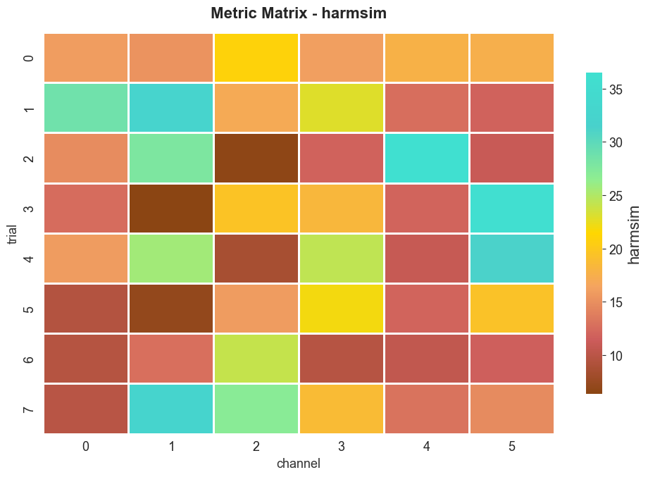
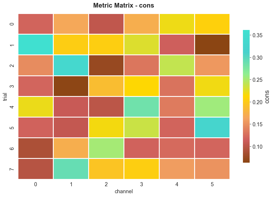
7. 3D group heatmaps

When the input is 3D (trials × channels × samples), BiotunerGroup exposes plot_metric_matrix, which renders metric values as a heatmap.

n_trials, n_ch = 8, 6
data_3d = np.array([
    [
        make_signal(
            [5 + rng.uniform(-0.5, 0.5),
             10 + rng.uniform(-0.5, 0.5),
             20 + rng.uniform(-1, 1)],
            [1.0, 0.7, 0.4],
            noise=0.1 + 0.05 * tr,
        )
        for _ in range(n_ch)
    ]
    for tr in range(n_trials)
])
print(f"3D data: {data_3d.shape}")

btg3 = BiotunerGroup(
    data_3d, sf=sf,
    axis_labels=["trial", "channel"],
    peaks_function="harmonic_recurrence",
    precision=0.25,
)
btg3.compute_peaks(min_freq=2, max_freq=50, n_peaks=5,
                   min_harms=2, verbose=False)
btg3.compute_metrics()
btg3.summary().head()

3D data: (8, 6, 8000)

C:\Users\skite\Documents\Github\biotuner\biotuner\metrics.py:946: RuntimeWarning: divide by zero encountered in scalar divide
  harm_temp.append(1 / delta_norm)

	trial	channel	series_idx	n_peaks	peak_freq_mean	peak_amp_mean	peak_freq_std	peak_amp_std	peak_freq_median	peak_amp_median	...	harm_pos_sem	subharm_tension	n_harmonic_recurrence	common_harm_pos	common_harm_pos_mean	common_harm_pos_std	common_harm_pos_median	common_harm_pos_min	common_harm_pos_max	common_harm_pos_sem
0	0	0	0	5	12.25	-26.493944	6.496153	21.793078	9.75	-42.435883	...	1.171771	0.019481	21	NaN	NaN	NaN	NaN	NaN	NaN	NaN
1	0	1	1	5	8.90	-26.447676	2.866182	21.615260	8.00	-43.653405	...	0.964203	0.014328	22	NaN	NaN	NaN	NaN	NaN	NaN	NaN
2	0	2	2	5	13.35	-26.588977	14.084211	21.891383	8.25	-41.786047	...	1.030776	0.0	25	NaN	NaN	NaN	NaN	NaN	NaN	NaN
3	0	3	3	5	8.95	-26.379970	3.508561	21.781310	8.50	-43.721270	...	1.030776	0.03544	25	NaN	NaN	NaN	NaN	NaN	NaN	NaN
4	0	4	4	5	9.35	-35.251479	5.791373	18.684407	8.00	-43.279380	...	1.006813	0.002496	27	5.0	NaN	NaN	NaN	NaN	NaN	NaN

5 rows × 36 columns

btg3.plot_metric_matrix(metric="harmsim")
plt.show()

btg3.plot_metric_matrix(metric="cons")
plt.show()

---

This walk-through covers the public plotting surface of biotuner. For the underlying analysis (peak extraction, tuning derivation, dissonance curve computation), see the Peaks extraction, Scale construction, and BiotunerGroup docs.