Chladni plates and spherical harmonics#

Eigenmodes of the wave equation on a bounded medium give standing-wave patterns whose nodal lines/surfaces fall on the points where the field is zero. harmonic_geometry exposes rectangular, circular, polygonal, and 3-D box plates, plus the spherical-harmonic basis on a sphere — the closed-surface analogue of a Chladni plate.

This notebook reproduces the plate and sphere figures from the report.

import warnings
from fractions import Fraction

import numpy as np
import matplotlib.pyplot as plt

from biotuner.harmonic_geometry import HarmonicInput, plotting

warnings.filterwarnings("ignore")
plt.rcParams["figure.dpi"] = 110

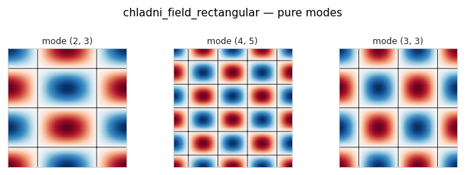
Rectangular plate — pure modes#

from biotuner.harmonic_geometry import chladni_field_rectangular

modes = [(2, 3), (4, 5), (3, 3)]
geoms = [chladni_field_rectangular([m], resolution=257) for m in modes]
plotting.gallery(geoms, titles=[f"mode {m}" for m in modes], n_cols=3,
                 suptitle="chladni_field_rectangular — pure modes");

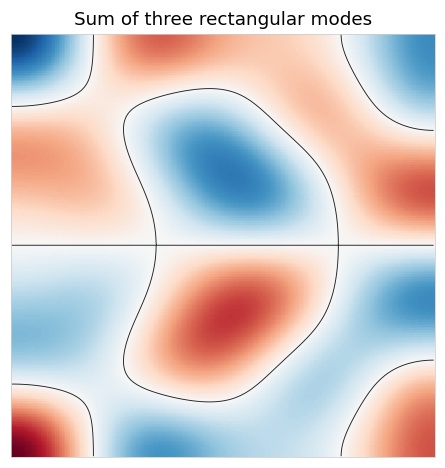
../../_images/80e2ca7f15527f56438ad4bc27b66a44f312465dbe9139d09c723c2a27e057f0.png

Superposition of modes#

Summing several modes with prescribed amplitudes and phases is what a real plate does under a chord-shaped excitation.

g = chladni_field_rectangular(
    modes=[(2, 3), (3, 5), (4, 1)],
    amps=[1.0, 0.6, 0.4],
    phases=[0.0, np.pi/3, np.pi/7],
    resolution=257,
)
fig, ax = plotting.plot_geometry(g)
ax.set_title("Sum of three rectangular modes");

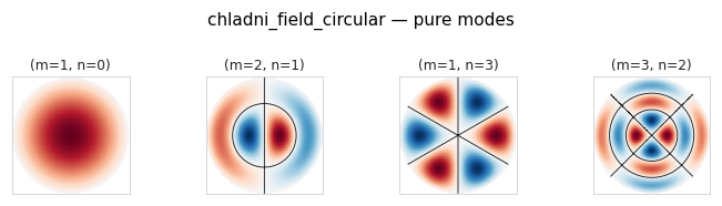
../../_images/e9122969a4eaa78f7f44563476e68c9e35e0690b2cac0bee2840ffeb42a76742.png

Circular plate (Bessel modes)#

from biotuner.harmonic_geometry import chladni_field_circular

cases = [([1], [0], "(m=1, n=0)"),
         ([2], [1], "(m=2, n=1)"),
         ([1], [3], "(m=1, n=3)"),
         ([3], [2], "(m=3, n=2)")]
geoms  = [chladni_field_circular(mr, ma, R=1.0, resolution=257) for mr, ma, _ in cases]
titles = [lab for _, _, lab in cases]
plotting.gallery(geoms, titles=titles, n_cols=4,
                 suptitle="chladni_field_circular — pure modes");

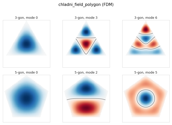
../../_images/780ce7486c907c06e70e45c5459b4dfd36f671e9a279fdbcad6339e990d90900.png

Polygonal plate (finite-difference)#

For arbitrary convex polygons the eigenproblem is solved on a finite difference mesh.

from biotuner.harmonic_geometry import chladni_field_polygon

cases = [(3, 0), (3, 3), (3, 6), (5, 0), (5, 2), (5, 5)]
geoms = [chladni_field_polygon([m], n_sides=ns, resolution=96)
         for ns, m in cases]
titles = [f"{ns}-gon, mode {m}" for ns, m in cases]
plotting.gallery(geoms, titles=titles, n_cols=3,
                 draw_kwargs={"show_nodal": True},
                 suptitle="chladni_field_polygon (FDM)");

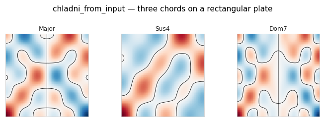
../../_images/44eb041f8269ca3224845f2f44175e50e2d24d6be1ab7f8f17876b9e32185239.png

From a chord input — `chladni_from_input`#

chladni_from_input ties a HarmonicInput chord to a plate: each ratio is mapped to a 2-D or 3-D mode index, the modes are summed, and the result is returned as a field_2d/field_3d GeometryData.

from biotuner.harmonic_geometry import chladni_from_input

chords = {
    "Major": HarmonicInput(ratios=[Fraction(1), Fraction(5, 4), Fraction(3, 2)]),
    "Sus4":  HarmonicInput(ratios=[Fraction(1), Fraction(4, 3), Fraction(3, 2)]),
    "Dom7":  HarmonicInput(ratios=[Fraction(1), Fraction(5, 4), Fraction(3, 2),
                                    Fraction(7, 4)]),
}
geoms = [chladni_from_input(c, plate="rectangular",
                             plate_kwargs={"resolution": 129})
         for c in chords.values()]
plotting.gallery(geoms, titles=list(chords.keys()), n_cols=3,
                 suptitle="chladni_from_input — three chords on a rectangular plate");

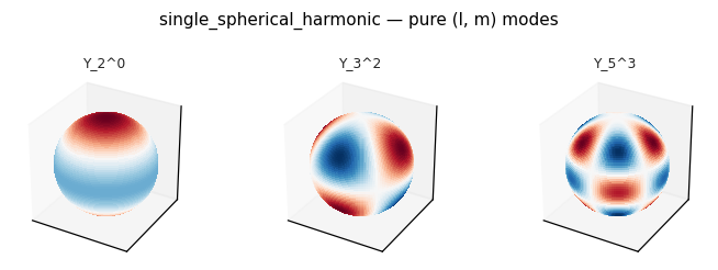
../../_images/8d75499263dbe5cc42fd7350b1277f06fc0d6dde1cee4dc91f272926f9d6738f.png

Spherical harmonics — closed-surface eigenmodes#

single_spherical_harmonic and spherical_harmonic_field produce the (l, m) eigenmodes of the Laplacian on the unit sphere. The plot below shows three pure modes rendered as colour on the sphere surface.

from biotuner.harmonic_geometry import single_spherical_harmonic

cases = [(2, 0), (3, 2), (5, 3)]
geoms  = [single_spherical_harmonic(l, m, n_theta=80, n_phi=160)
          for l, m in cases]
titles = [f"Y_{l}^{m}" for l, m in cases]
plotting.gallery(geoms, titles=titles, n_cols=3,
                 suptitle="single_spherical_harmonic — pure (l, m) modes");

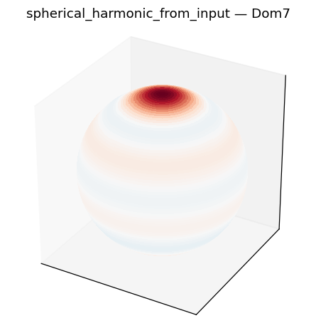
../../_images/bcc7bd8249c7efa6512d7a512507ee8f4e008534c79a9341f9f9428428ff77ce.png

Chord on a sphere#

from biotuner.harmonic_geometry import spherical_harmonic_from_input

dom7 = HarmonicInput(ratios=[Fraction(1), Fraction(5, 4),
                              Fraction(3, 2), Fraction(7, 4)])
g = spherical_harmonic_from_input(dom7, n_theta=96, n_phi=192)
fig, ax = plotting.plot_geometry(g)
ax.set_title("spherical_harmonic_from_input — Dom7");

../../_images/4a573c960f4cb2d334c1055244d0e0f71f85f5193765ac215cfdda0f2f4c7a16.png

Chladni plates and spherical harmonics

Contents