Eigenmode and wave-field media#
The eigenmode family solves a bounded standing-wave eigenproblem and
returns the chord-weighted superposition of the eigenmodes; the
wave_field family superposes coherent travelling waves on an unbounded
medium.
Same chord set, two very different physics.
import warnings
from fractions import Fraction

import numpy as np
import matplotlib.pyplot as plt

from biotuner.harmonic_geometry import HarmonicInput, plotting

warnings.filterwarnings("ignore")
plt.rcParams["figure.dpi"] = 110

# A small reference set of chord inputs used across the notebook.
CHORDS = {
    "Major": HarmonicInput(ratios=[Fraction(1), Fraction(5, 4), Fraction(3, 2)]),
    "Sus4":  HarmonicInput(ratios=[Fraction(1), Fraction(4, 3), Fraction(3, 2)]),
    "Dom7":  HarmonicInput(ratios=[Fraction(1), Fraction(5, 4),
                                    Fraction(3, 2), Fraction(7, 4)]),
    "Dim7":  HarmonicInput(ratios=[Fraction(1), Fraction(6, 5),
                                    Fraction(7, 5), Fraction(12, 7)]),
}
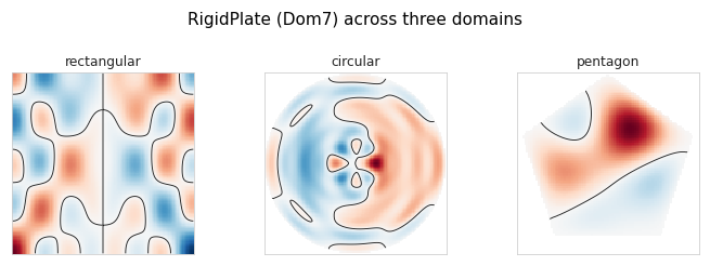
Eigenmode — RigidPlate across three domains#
from biotuner.harmonic_geometry.media import (
    RigidPlate, ClosedSurface, Elastic, PlasmaLattice,
    Rectangular, Circular, PolygonDomain,
)

geoms = [
    RigidPlate(domain=Rectangular(),               resolution=128)(CHORDS["Dom7"]),
    RigidPlate(domain=Circular(R=1.0),             resolution=128)(CHORDS["Dom7"]),
    RigidPlate(domain=PolygonDomain(n_sides=5),    resolution=96)(CHORDS["Dom7"]),
]
plotting.gallery(geoms,
                 titles=["rectangular", "circular", "pentagon"],
                 n_cols=3,
                 suptitle="RigidPlate (Dom7) across three domains");
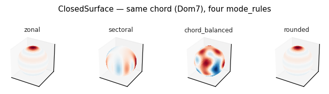
Eigenmode — ClosedSurface on a sphere (chord-driven Y_lm modes)#
The default mode_rule='zonal' uses only $(l, 0)$ modes, which have no
longitudinal variation — the sphere lights up symmetrically around the
poles. The other three rules expose richer chord-dependent geometry:
sectoral— uses $|m| = l$ (banana-shaped equatorial lobes)chord_balanced— mixes $m \in {0, ±1, …, ±l}$ across componentsrounded— rounds $m$ proportional to the ratio magnitude
# Side-by-side comparison: same chord, four mode_rules
sphere_rules = ["zonal", "sectoral", "chord_balanced", "rounded"]
geoms = [ClosedSurface(mode_rule=r, max_l=12,
                        n_theta=96, n_phi=192)(CHORDS["Dom7"])
         for r in sphere_rules]
plotting.gallery(geoms, titles=sphere_rules, n_cols=4,
                 suptitle="ClosedSurface — same chord (Dom7), four mode_rules");
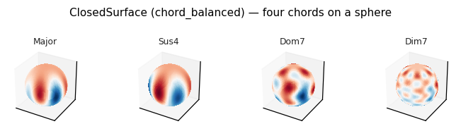
# Four chords, rendered with the visually richest mode_rule.
sphere = ClosedSurface(mode_rule="chord_balanced", max_l=12,
                       n_theta=96, n_phi=192)
geoms  = [sphere(CHORDS[n]) for n in CHORDS]
plotting.gallery(geoms, titles=list(CHORDS.keys()), n_cols=4,
                 suptitle="ClosedSurface (chord_balanced) — four chords on a sphere");
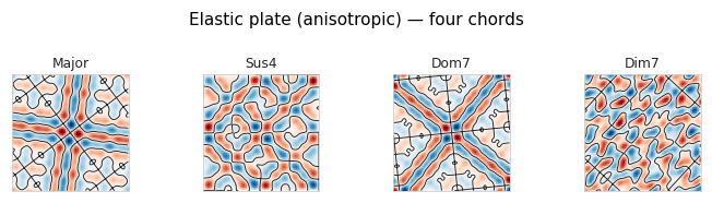
Eigenmode — Elastic (anisotropy in the wave operator)#
Elastic solves the elastic-wave eigenproblem on a rectangular domain
with an optional anisotropy axis. The fundamental mode is then
chord-modulated.
elastic = Elastic(resolution=160, n_modes=24)
geoms   = [elastic(CHORDS[n]) for n in CHORDS]
plotting.gallery(geoms, titles=list(CHORDS.keys()), n_cols=4,
                 suptitle="Elastic plate (anisotropic) — four chords");
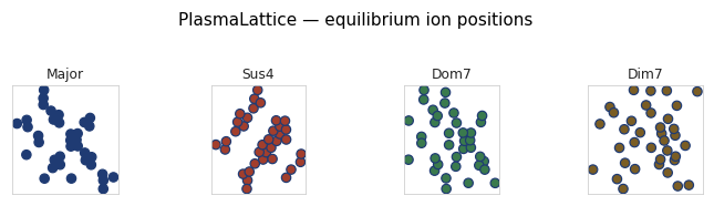
Eigenmode — PlasmaLattice (chord-tuned ion crystal)#
A relaxed Coulomb crystal where the trapping potential is modulated by the chord ratios; the medium returns the equilibrium ion positions as a 2-D point cloud.
lattice = PlasmaLattice(n_ions=36, n_steps=200,
                         chord_resolution=128, rng_seed=0)
geoms   = [lattice(CHORDS[n]) for n in CHORDS]
plotting.gallery(geoms, titles=list(CHORDS.keys()), n_cols=4,
                 suptitle="PlasmaLattice — equilibrium ion positions");
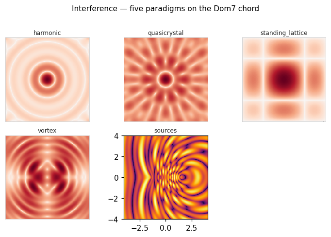
Wave-field — Interference (five paradigms)#
Interference is a thin facade around the five travelling-wave
paradigms exposed in :mod:harmonic_geometry.interference_patterns.
The same chord becomes five visually distinct fields.
from biotuner.harmonic_geometry.media import Interference

paradigms = ["harmonic", "quasicrystal", "standing_lattice", "vortex", "sources"]
geoms = [Interference(paradigm=p, resolution=192)(CHORDS["Dom7"])
         for p in paradigms]
plotting.gallery(geoms, titles=paradigms, n_cols=3,
                 suptitle="Interference — five paradigms on the Dom7 chord");
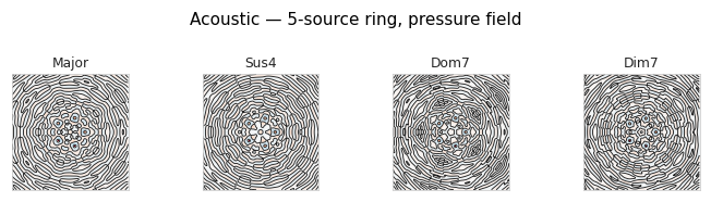
Wave-field — Acoustic (multi-source pressure field)#
Acoustic places n_sources emitters on a configurable layout (a ring
by default), assigns one chord component per source, and superposes the
resulting outgoing pressure waves.
from biotuner.harmonic_geometry.media import Acoustic

acoustic = Acoustic(n_sources=5, source_layout="ring", resolution=224,
                    base_frequency=8.0)
geoms = [acoustic(CHORDS[n]) for n in CHORDS]
plotting.gallery(geoms, titles=list(CHORDS.keys()), n_cols=4,
                 suptitle="Acoustic — 5-source ring, pressure field");