The media subpackage: medium protocol, domains, pipelines

biotuner.harmonic_geometry.media is a family of chord-driven response operators. Every medium implements respond(forcing) → GeometryData where the forcing is either a :class:HarmonicInput (a chord) or a pre-computed :class:GeometryData (a wave field), and the output is one of the standard geometry types — typically a 2-D field, a point cloud, or a vector field.

Media are organised into five families:

family	what it does
eigenmode	bounded standing-wave eigenproblem (plate / sphere / elastic / ion lattice)
wave_field	open-medium coherent superposition (interference / acoustic)
parametric	parametric-instability surface (Faraday, cymatics)
transport	passive redistribution on an existing wave field (Granular, Tracer, Streaming)
morphogenetic	pattern growth shaped by a chord (Crystallization, Reaction-Diffusion)

This notebook walks through the protocol, the available Domain types, and how to compose media into pipelines.

import warnings
from fractions import Fraction

import numpy as np
import matplotlib.pyplot as plt

from biotuner.harmonic_geometry import HarmonicInput, plotting

warnings.filterwarnings("ignore")
plt.rcParams["figure.dpi"] = 110

# A small reference set of chord inputs used across the notebook.
CHORDS = {
    "Major": HarmonicInput(ratios=[Fraction(1), Fraction(5, 4), Fraction(3, 2)]),
    "Sus4":  HarmonicInput(ratios=[Fraction(1), Fraction(4, 3), Fraction(3, 2)]),
    "Dom7":  HarmonicInput(ratios=[Fraction(1), Fraction(5, 4),
                                    Fraction(3, 2), Fraction(7, 4)]),
    "Dim7":  HarmonicInput(ratios=[Fraction(1), Fraction(6, 5),
                                    Fraction(7, 5), Fraction(12, 7)]),
}

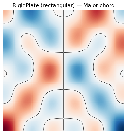
A single medium — respond(chord) returns a GeometryData

from biotuner.harmonic_geometry.media import RigidPlate, Rectangular

plate = RigidPlate(domain=Rectangular(Lx=1.0, Ly=1.0), resolution=128)
g     = plate.respond(CHORDS["Major"])
print("output geom_type:", g.geom_type)
print("output kind:     ", (g.metadata or {}).get("kind"))
print("output shape:    ", np.asarray(g.coordinates).shape)

fig, ax = plotting.plot_geometry(g)
ax.set_title("RigidPlate (rectangular) — Major chord");

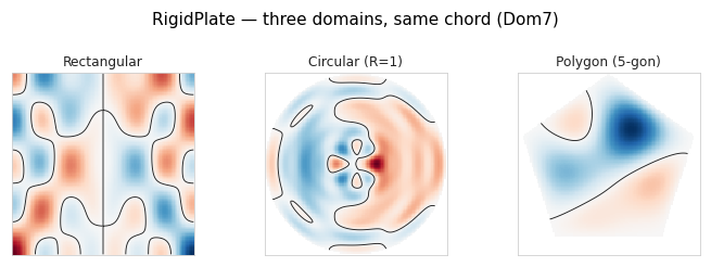
Domains — change the boundary, keep the chord

Rectangular, Circular, PolygonDomain, Box3D, and Sphere swap in without touching the medium’s other parameters.

from biotuner.harmonic_geometry.media import Circular, PolygonDomain

domains = [
    ("Rectangular",         Rectangular(Lx=1.0, Ly=1.0)),
    ("Circular (R=1)",      Circular(R=1.0)),
    ("Polygon (5-gon)",     PolygonDomain(n_sides=5, radius=1.0)),
]
geoms = [RigidPlate(domain=d, resolution=128)(CHORDS["Dom7"])
         for _, d in domains]
plotting.gallery(geoms, titles=[name for name, _ in domains], n_cols=3,
                 suptitle="RigidPlate — three domains, same chord (Dom7)");

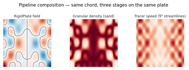
Pipelines — chain media

Pipeline(A, B, C)(chord) is equivalent to C(B(A(chord))), with the correct forcing type negotiated at each stage. Below we feed a plate field into the Granular transport medium (sand on a vibrating plate) and into the Tracer flow medium (light particles advected by ∇² streamlines of the field).

from biotuner.harmonic_geometry.media import Pipeline, Granular, Tracer

plate    = RigidPlate(domain=Rectangular(), resolution=160)
sand     = Pipeline(plate, Granular(n_particles=3000, output_mode="density"))
flow     = Pipeline(plate, Tracer(output_mode="speed"))

geoms = [plate(CHORDS["Dom7"]),
         sand (CHORDS["Dom7"]),
         flow (CHORDS["Dom7"])]
plotting.gallery(
    geoms,
    titles=["RigidPlate field", "Granular density (sand)",
            "Tracer speed (∇² streamlines)"],
    n_cols=3,
    suptitle="Pipeline composition — same chord, three stages on the same plate",
);

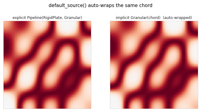
default_source — transport / morphogenetic media auto-wrap

Granular, Tracer, Streaming, Crystallization, and ReactionDiffusion declare a default_source() so they accept a :class:HarmonicInput directly: the medium silently wraps the chord through its default upstream medium. The Granular default is a square :class:RigidPlate, so the two snippets below are equivalent.

# Explicit two-stage pipeline:
explicit = Pipeline(RigidPlate(), Granular(n_particles=3000))(CHORDS["Sus4"])

# Implicit: pass a chord straight to Granular and let it auto-wrap.
implicit = Granular(n_particles=3000)(CHORDS["Sus4"])

plotting.gallery([explicit, implicit],
                 titles=["explicit Pipeline(RigidPlate, Granular)",
                         "implicit Granular(chord)  (auto-wrapped)"],
                 n_cols=2,
                 suptitle="default_source() auto-wraps the same chord");