Parametric and transport media

Faraday is a parametric-instability surface: the chord ratios pick the unstable wave-numbers via a Mathieu-style dispersion, and the resulting pattern is a chord-tuned cymatics image. The transport family then takes a wave field (or a chord, auto-wrapped) and redistributes mass or flow on top of it — sand grains piling on the nodes (Granular), tracer particles flowing along the gradient streamlines (Tracer), acoustic streaming velocities (Streaming).

import warnings
from fractions import Fraction

import numpy as np
import matplotlib.pyplot as plt

from biotuner.harmonic_geometry import HarmonicInput, plotting

warnings.filterwarnings("ignore")
plt.rcParams["figure.dpi"] = 110

# A small reference set of chord inputs used across the notebook.
CHORDS = {
    "Major": HarmonicInput(ratios=[Fraction(1), Fraction(5, 4), Fraction(3, 2)]),
    "Sus4":  HarmonicInput(ratios=[Fraction(1), Fraction(4, 3), Fraction(3, 2)]),
    "Dom7":  HarmonicInput(ratios=[Fraction(1), Fraction(5, 4),
                                    Fraction(3, 2), Fraction(7, 4)]),
    "Dim7":  HarmonicInput(ratios=[Fraction(1), Fraction(6, 5),
                                    Fraction(7, 5), Fraction(12, 7)]),
}

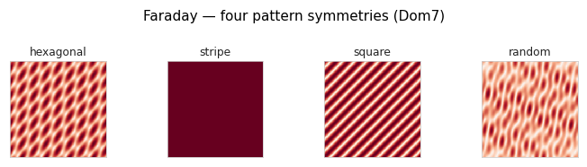
Faraday — chord-tuned cymatics patterns

from biotuner.harmonic_geometry.media import Faraday

patterns = ["hexagonal", "stripe", "square", "random"]
geoms = [Faraday(pattern=p, resolution=192, seed=0)(CHORDS["Dom7"])
         for p in patterns]
plotting.gallery(geoms, titles=patterns, n_cols=4,
                 suptitle="Faraday — four pattern symmetries (Dom7)");

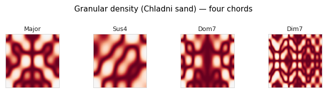
Granular — sand-on-plate density across chords

from biotuner.harmonic_geometry.media import Granular, RigidPlate, Pipeline

# Auto-wrap: Granular's default_source is a square RigidPlate.
geoms = [Granular(n_particles=3000, output_mode="density",
                   seed=0)(CHORDS[n]) for n in CHORDS]
plotting.gallery(geoms, titles=list(CHORDS.keys()), n_cols=4,
                 suptitle="Granular density (Chladni sand) — four chords");

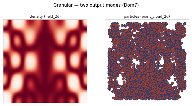
Same chord, two output modes

output_mode="density" returns a smoothed 2-D density field; output_mode="particles" returns the raw scatter.

g_density   = Granular(n_particles=4000, output_mode="density",   seed=0)(CHORDS["Dom7"])
g_particles = Granular(n_particles=4000, output_mode="particles", seed=0)(CHORDS["Dom7"])
plotting.gallery([g_density, g_particles],
                 titles=["density (field_2d)", "particles (point_cloud_2d)"],
                 n_cols=2,
                 suptitle="Granular — two output modes (Dom7)");

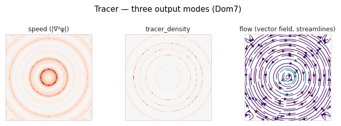
Tracer — flow streamlines on a wave field

Tracer returns either a speed map (output_mode='speed'), a tracer density (output_mode='tracer_density'), or the raw 2-D vector field itself (output_mode='flow'). The vector-field output is rendered with the new draw_vector_field_2d helper in :mod:harmonic_geometry.plotting — streamlines on a magma background proportional to the local flow magnitude.

from biotuner.harmonic_geometry.media import Tracer

t_speed   = Tracer(output_mode="speed")(CHORDS["Dom7"])
t_density = Tracer(output_mode="tracer_density")(CHORDS["Dom7"])
t_flow    = Tracer(output_mode="flow")(CHORDS["Dom7"])

plotting.gallery([t_speed, t_density, t_flow],
                 titles=["speed (|∇²ψ|)", "tracer_density",
                         "flow (vector field, streamlines)"],
                 n_cols=3,
                 suptitle="Tracer — three output modes (Dom7)");

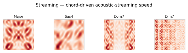
Streaming — acoustic-streaming velocity magnitude

from biotuner.harmonic_geometry.media import Streaming

geoms = [Streaming(output_mode="speed")(CHORDS[n]) for n in CHORDS]
plotting.gallery(geoms, titles=list(CHORDS.keys()), n_cols=4,
                 suptitle="Streaming — chord-driven acoustic-streaming speed");