Chladni cymatics — chord-driven nodal patterns#

The Chladni sand-on-square-plate experiment is the canonical visual representation of musical chord ratios. Sand grains settle on the nodal lines of a vibrating plate — the curves where the plate’s displacement is zero. Different chord ratios excite different combinations of plate eigenmodes and the resulting nodal lattice becomes a unique “fingerprint” for each chord.

RigidPlate (the eigenmode-family medium in :mod:biotuner.harmonic_geometry.media) exposes two parallel paths:

classical (default) — mode_scheme='per_ratio': each ratio maps to one (m, n) mode pair via Stern-Brocot, and the field is a sum of symmetric cos·cos products. Works on rectangular, circular, polygonal, and 3-D-box plates.
cymatics (new) — mode_scheme='pairwise_antisymmetric': each pair of ratios contributes one antisymmetric mode cos(m)cos(n) - cos(n)cos(m) on a square plate. This is the iconic Chladni form. Rectangular only.

This notebook walks through the cymatics path: integer-ratio extraction, the four mode-scheme options, D4 symmetrisation, the nodal-density transform, two rendering styles (white-sand particles and a perceptual-cmap “painted” view), the max_mode cap that tames chords with high LCMs, and finally an animation that morphs through a sequence of chords.

import warnings
from fractions import Fraction

import numpy as np
import matplotlib.pyplot as plt

from biotuner.harmonic_geometry import HarmonicInput, plotting
from biotuner.harmonic_geometry.media import (
    Granular, Pipeline, RigidPlate,
)
from biotuner.harmonic_geometry.media.eigenmode.rigid_plate import (
    chord_to_int_modes,
    chladni_field_pairwise,
    chladni_field_triple_antisymmetric,
    chladni_nodal_density,
)

warnings.filterwarnings("ignore")
plt.rcParams["figure.dpi"] = 110

# Small-integer just-intoned chord representations — the natural form
# for the cymatics schemes (one chord ratio = one plate wavenumber).
CHORDS_INT = {
    "Major":  [4, 5, 6],
    "Sus4":   [6, 8, 9],
    "Dom7":   [4, 5, 6, 7],
    "Dim7":   [5, 6, 7, 9],
}

1. Lossless integer-ratio extraction#

chord_to_int_modes multiplies a chord’s Fraction ratios through by the LCM of their denominators. No rounding. Just-intoned chords already in small-integer form round-trip unchanged; 12-TET-flavoured forms can produce surprisingly large integers.

chords_frac = {
    "Major":  [Fraction(1), Fraction(5, 4), Fraction(3, 2)],
    "Dom7":   [Fraction(1), Fraction(5, 4), Fraction(3, 2), Fraction(7, 4)],
    "Dim7-just":  [Fraction(1), Fraction(6, 5), Fraction(7, 5), Fraction(9, 5)],
    "Dim7-12TET": [Fraction(1), Fraction(6, 5), Fraction(7, 5), Fraction(12, 7)],
}
for name, c in chords_frac.items():
    print(f"  {name:12s}  {[str(r) for r in c]}  →  {chord_to_int_modes(c)}")

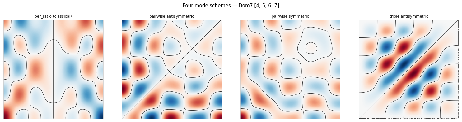
2. The four mode schemes#

RigidPlate exposes four chord→mode schemes. The classical per_ratio lives next to three cymatics-style schemes that sum modes over pairs or triples of ratios — emphasising the harmonic relationships in the chord rather than the individual partials.

dom7_int = CHORDS_INT["Dom7"]
dom7_hi  = HarmonicInput(ratios=[Fraction(r, 4) for r in dom7_int])

g_pr = RigidPlate(mode_scheme="per_ratio", resolution=400)(dom7_hi)
g_pa = chladni_field_pairwise(dom7_int, antisymmetric=True,  resolution=400)
g_ps = chladni_field_pairwise(dom7_int, antisymmetric=False, resolution=400)
g_tr = chladni_field_triple_antisymmetric(dom7_int, resolution=400)

plotting.gallery(
    [g_pr, g_pa, g_ps, g_tr], n_cols=4,
    titles=["per_ratio (classical)",
            "pairwise antisymmetric",
            "pairwise symmetric",
            "triple antisymmetric"],
    suptitle="Four mode schemes — Dom7 [4, 5, 6, 7]",
    fig_width=14.0,
);

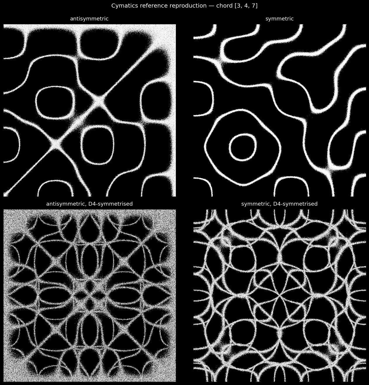
../../_images/3333d2204b371ae279e1cace78c5c30b29dd433037a0b917ce6b7bf1405f1312.png

3. D4 symmetrisation — applied at the density stage#

The classical Chladni demos apply D4 (4-fold rotational + reflective) symmetrisation to the density exp(-w²/σ²), taking the element-wise max over the 8-element orbit. This unions the nodal sets across rotations — producing the rich crystalline lattice the cymatics aesthetic is known for. RigidPlate(symmetry='d4_max') records the request; chladni_nodal_density (and the Granular(nodal_emphasis=True) path) then applies it at the density stage.

chord = [3, 4, 7]  # the user's original cymatics-demo chord

fig, axes = plt.subplots(2, 2, figsize=(12, 12), facecolor="black")
configs = [
    ("antisymmetric",                  True,  "none"),
    ("symmetric",                      False, "none"),
    ("antisymmetric, D4-symmetrised",  True,  "d4_max"),
    ("symmetric, D4-symmetrised",      False, "d4_max"),
]
for ax, (label, asy, sym) in zip(axes.flat, configs):
    field = chladni_field_pairwise(
        chord, antisymmetric=asy, symmetry=sym,
        resolution=400, pair_subset="all",
    )
    plotting.draw_chladni_sand(field, ax, n_particles=300_000,
                                point_size=0.4, point_alpha=0.4,
                                sigma=0.05)
    ax.set_title(label, color="white", fontsize=12, pad=8)
fig.suptitle(f"Cymatics reference reproduction — chord {chord}",
             color="white", fontsize=13, y=0.995)
fig.tight_layout();

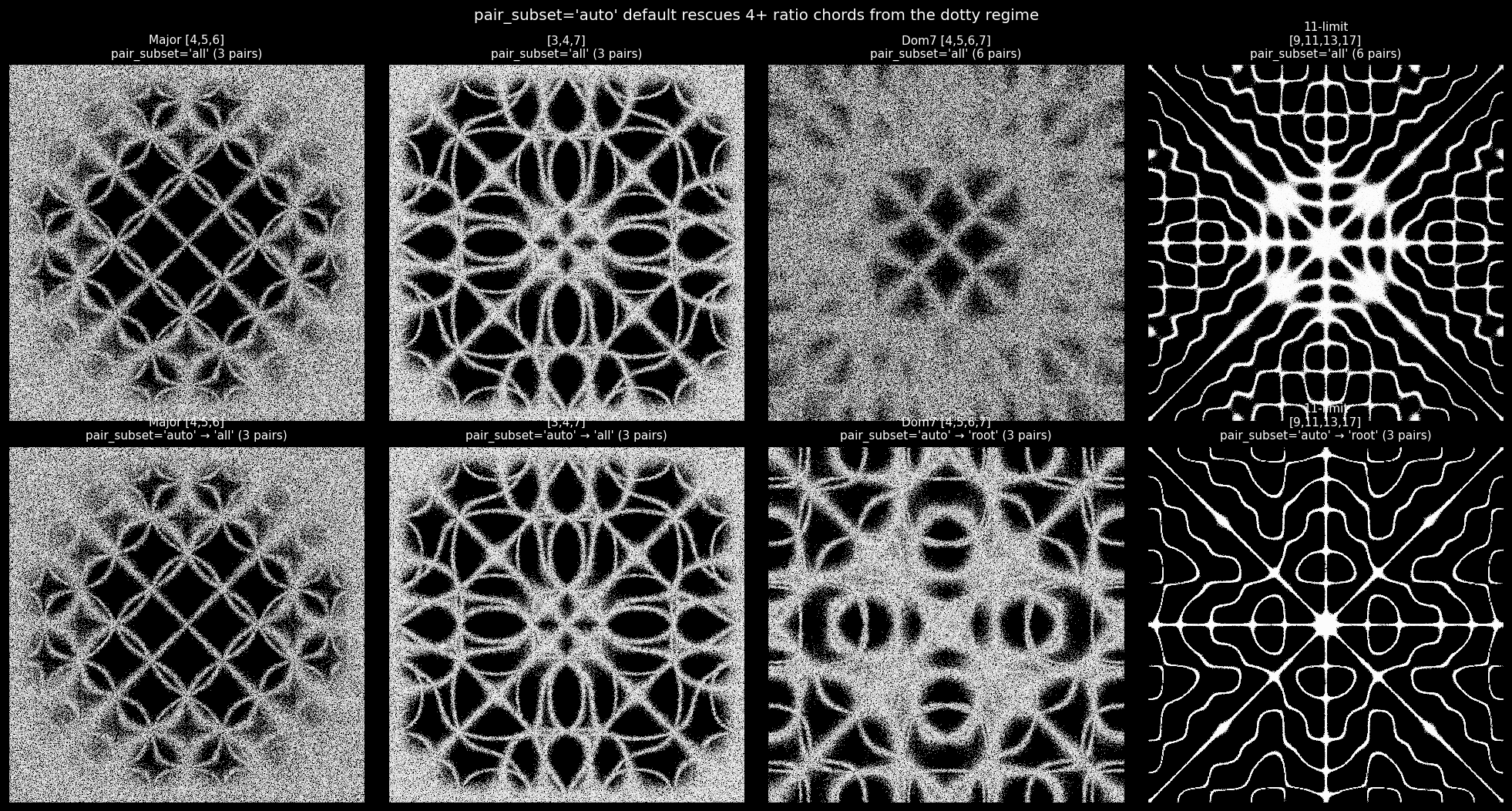
../../_images/2f362ce6730439859bfa201a65b8a19c30332cfe13da1cb468dc6a94c420c63c.png

4. `pair_subset` — keeping curves bold at any chord size#

Summing all C(n, 2) pair-modes produces continuous curves for 3-ratio chords (the simultaneous zero-set is a curve) but degenerates into a set of isolated points for 4+ ratio chords (the simultaneous zero-set becomes restrictive). The pair_subset parameter exposes the workaround: keep only n-1 pairs and the field stays curve-like at any chord size.

pair_subset='auto' (default): 'all' for n ≤ 3, 'root' for n ≥ 4.
'all': literal mathematical sum (dotty for n ≥ 4).
'adjacent': consecutive pairs.
'root': pairs that include the first ratio.
list of (m, n) tuples: full manual control.

fig, axes = plt.subplots(2, 4, figsize=(18, 9.5), facecolor="black")
chords = [
    ("Major [4,5,6]",        [4, 5, 6]),
    ("[3,4,7]",              [3, 4, 7]),
    ("Dom7 [4,5,6,7]",       [4, 5, 6, 7]),
    ("11-limit\n[9,11,13,17]", [9, 11, 13, 17]),
]
for ax, (name, chord) in zip(axes[0], chords):
    f = chladni_field_pairwise(
        chord, antisymmetric=True, symmetry="d4_max",
        resolution=400, pair_subset="all",
    )
    plotting.draw_chladni_sand(f, ax, n_particles=300_000,
                                point_size=0.4, point_alpha=0.4)
    n = f.parameters["n_pairs"]
    ax.set_title(f"{name}\npair_subset='all' ({n} pairs)",
                  color="white", fontsize=10)
for ax, (name, chord) in zip(axes[1], chords):
    f = chladni_field_pairwise(
        chord, antisymmetric=True, symmetry="d4_max",
        resolution=400,  # pair_subset='auto'
    )
    plotting.draw_chladni_sand(f, ax, n_particles=300_000,
                                point_size=0.4, point_alpha=0.4)
    actual = f.parameters["pair_subset"]
    n = f.parameters["n_pairs"]
    ax.set_title(f"{name}\npair_subset='auto' → '{actual}' ({n} pairs)",
                  color="white", fontsize=10)
fig.suptitle("pair_subset='auto' default rescues 4+ ratio chords from the dotty regime",
             color="white", fontsize=13, y=0.995)
fig.tight_layout(pad=0.6);

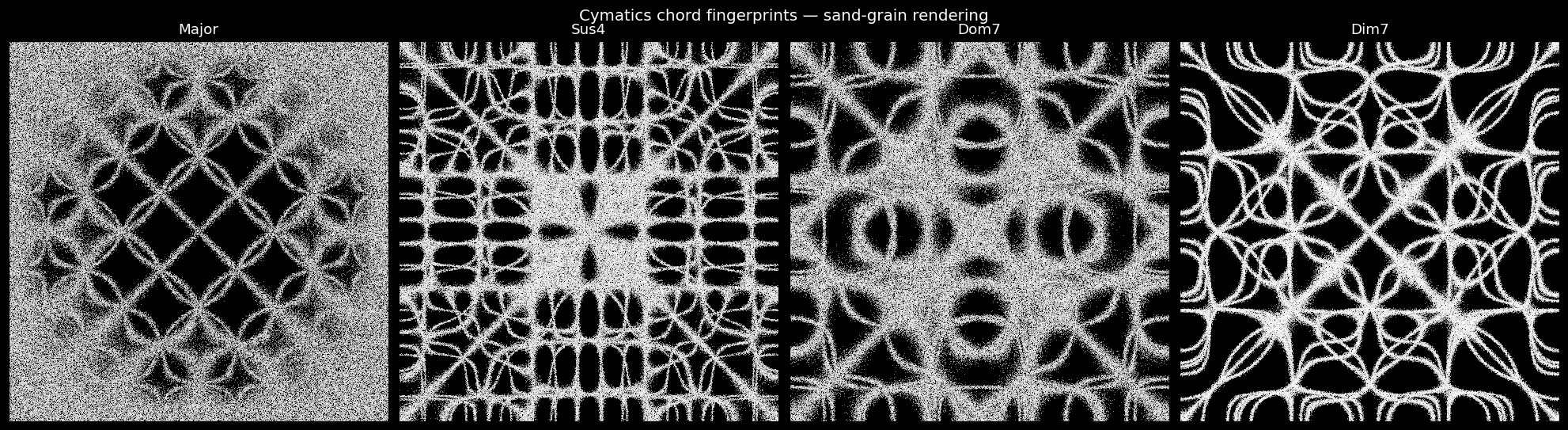
../../_images/473e04179197a4863fc59feaca4680248a7a861f76b7b446db1897916712ceff.png

5. Chord-fingerprint gallery — sand-grain rendering#

plotting.draw_chladni_sand density-samples n_particles points from the nodal density and renders them as a black-plate / white-grain scatter — the photographic Chladni look. Auto-σ from the chord metadata.

fig, axes = plt.subplots(1, 4, figsize=(18, 4.7), facecolor="black")
for ax, (name, chord) in zip(axes, CHORDS_INT.items()):
    field = chladni_field_pairwise(
        chord, antisymmetric=True, symmetry="d4_max",
        resolution=400,
    )
    plotting.draw_chladni_sand(field, ax, n_particles=300_000,
                                point_size=0.4, point_alpha=0.4)
    ax.set_title(name, color="white", fontsize=12)
fig.suptitle("Cymatics chord fingerprints — sand-grain rendering",
             color="white", fontsize=13, y=1.02)
fig.tight_layout(pad=0.4);

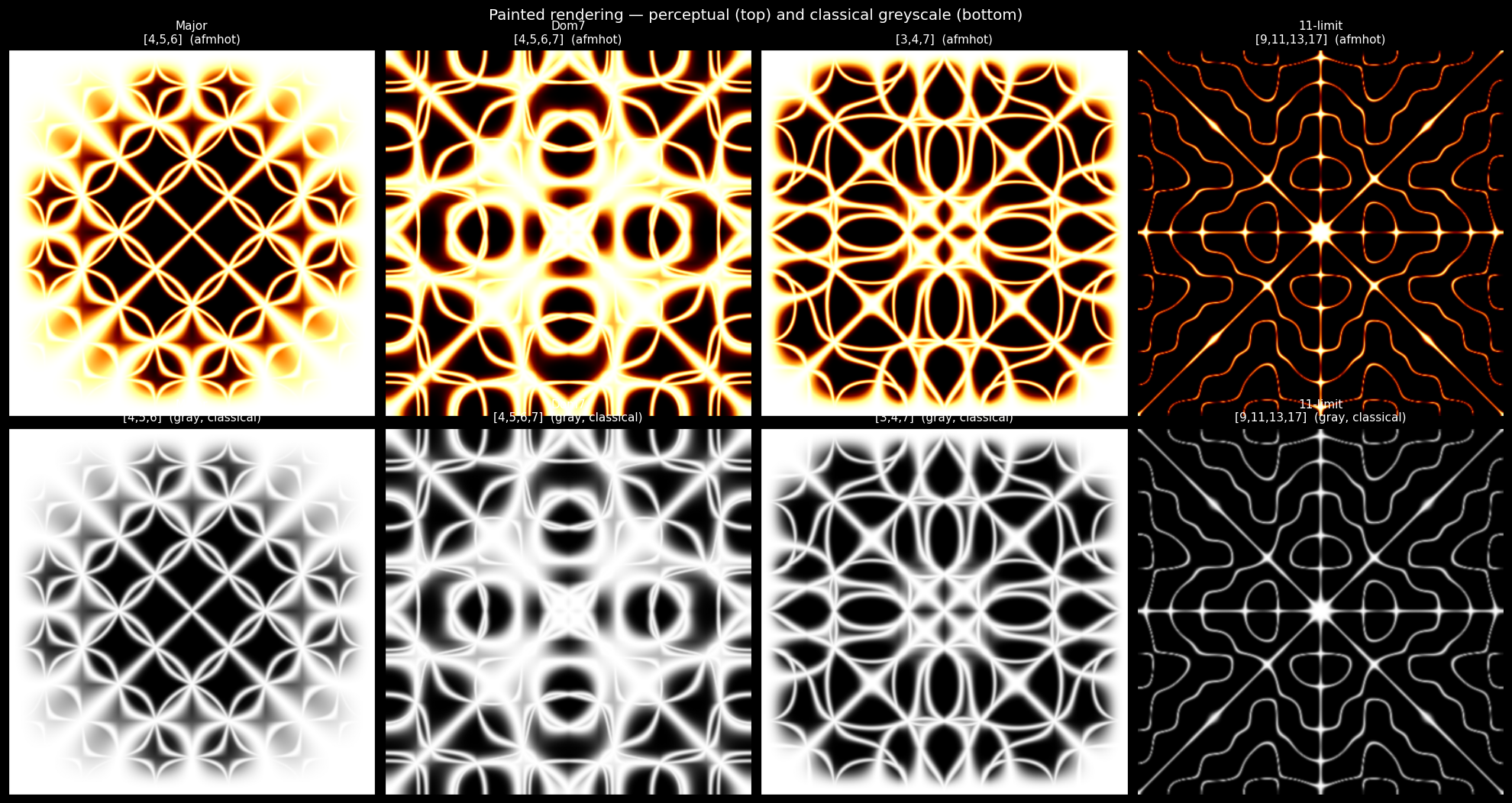
../../_images/cbffd808fe9826819c5d5bd0c35796487810cd694ded1f53da9f458cb2e5cbf6.png

6. Painted rendering — perceptual cmap alternative#

plotting.draw_chladni_painted renders the same density via imshow on a perceptual luminance ramp (afmhot by default), or greyscale for the classical look. Faster than the particle sampler and well suited to high-wavenumber chords where individual grains get lost.

fig, axes = plt.subplots(2, 4, figsize=(18, 9.5), facecolor="black")
chords_gamut = [
    ("Major\n[4,5,6]",    [4, 5, 6]),
    ("Dom7\n[4,5,6,7]",   [4, 5, 6, 7]),
    ("[3,4,7]",            [3, 4, 7]),
    ("11-limit\n[9,11,13,17]", [9, 11, 13, 17]),
]
for ax, (name, chord) in zip(axes[0], chords_gamut):
    f = chladni_field_pairwise(
        chord, antisymmetric=True, symmetry="d4_max", resolution=400,
    )
    plotting.draw_chladni_painted(f, ax, cmap="afmhot", gamma=0.85)
    ax.set_title(f"{name}  (afmhot)", color="white", fontsize=10)
for ax, (name, chord) in zip(axes[1], chords_gamut):
    f = chladni_field_pairwise(
        chord, antisymmetric=True, symmetry="d4_max", resolution=400,
    )
    plotting.draw_chladni_painted(f, ax, cmap="gray", gamma=0.55)
    ax.set_title(f"{name}  (gray, classical)", color="white", fontsize=10)
fig.suptitle("Painted rendering — perceptual (top) and classical greyscale (bottom)",
             color="white", fontsize=13, y=0.995)
fig.tight_layout(pad=0.6);

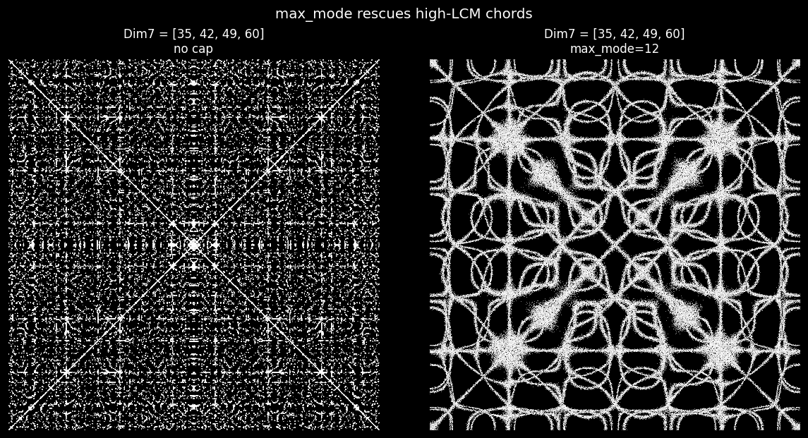
../../_images/54f11d9f3349d72674300d95430e7bd3f27cb341f2a47b82c722fb4512c464d1.png

7. `max_mode` — taming high-LCM chords#

Chords whose Fraction form has a large LCM (e.g. 12-TET-flavoured Dim7 = [35, 42, 49, 60]) produce sub-pixel-fine lattices that read as dots rather than curves. max_mode scales all wavenumbers proportionally down to a visible range — ratios are preserved.

dim7_blown = [35, 42, 49, 60]
fig, axes = plt.subplots(1, 2, figsize=(11, 5.6), facecolor="black")
for ax, cap in zip(axes, [None, 12]):
    f = chladni_field_pairwise(
        dim7_blown, antisymmetric=True, symmetry="d4_max",
        resolution=480, max_mode=cap,
    )
    plotting.draw_chladni_sand(f, ax, n_particles=300_000,
                                point_size=0.4, point_alpha=0.4)
    title = "no cap" if cap is None else f"max_mode={cap}"
    ax.set_title(f"Dim7 = {dim7_blown}\n{title}",
                  color="white", fontsize=11)
fig.suptitle("max_mode rescues high-LCM chords",
             color="white", fontsize=13, y=1.0)
fig.tight_layout();

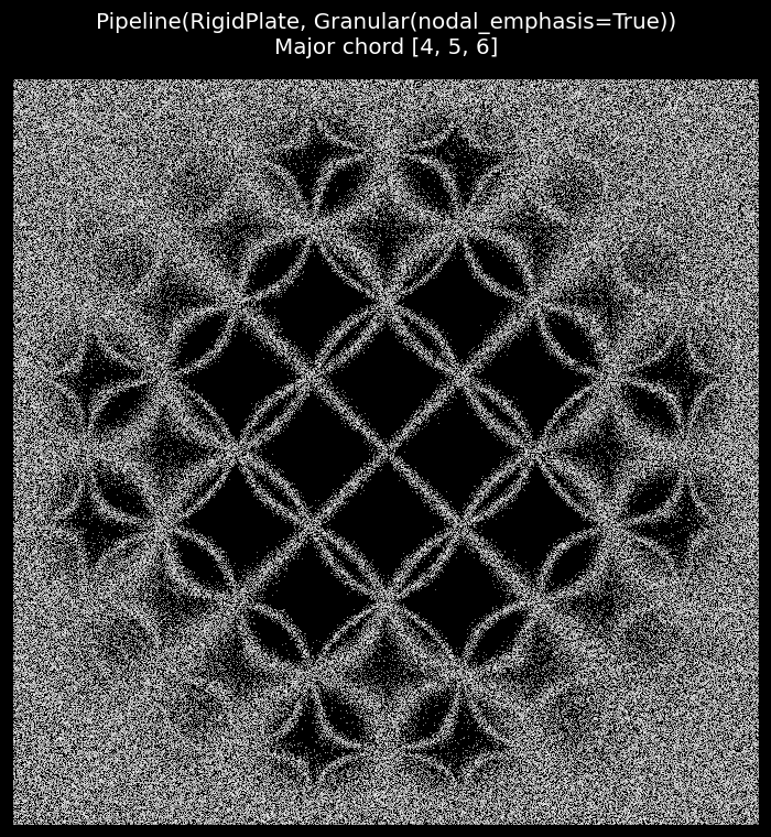
../../_images/62dce9004cbe4ca020e9b9e8faad735bacde1c6532633e76c091cf60a325e48e.png

8. Pipeline composition: `RigidPlate → Granular`#

The Granular transport medium picks up a wave field and samples a density-weighted point cloud. With nodal_emphasis=True it uses exp(-w²/σ²) directly on the input field (auto-σ from metadata) and applies any D4 symmetrisation from the upstream RigidPlate.symmetry setting. So the entire cymatics flow becomes a clean Pipeline:

pipeline = Pipeline(
    RigidPlate(mode_scheme="pairwise_antisymmetric",
               symmetry="d4_max", resolution=400),
    Granular(output_mode="particles", nodal_emphasis=True,
             n_particles=400_000, seed=0),
)
chord = HarmonicInput(ratios=[Fraction(4), Fraction(5), Fraction(6)])
result = pipeline(chord)

fig, ax = plt.subplots(figsize=(7, 7), facecolor="black")
ax.set_facecolor("black")
pts = result.coordinates
ax.scatter(pts[:, 0], pts[:, 1], s=0.4, c="white", alpha=0.4, linewidths=0)
ax.set_aspect("equal"); ax.set_xticks([]); ax.set_yticks([])
ax.set_xlim(0, 1); ax.set_ylim(0, 1)
fig.suptitle("Pipeline(RigidPlate, Granular(nodal_emphasis=True))\nMajor chord [4, 5, 6]",
             color="white", fontsize=13)
fig.tight_layout();

../../_images/5d23b3078e6239370df11704f3d08fe8da394e431f43032bc6c3c0af3c35d4c8.png

9. Animation — chord-sequence morph#

plotting.animate_chord_sequence drives a user-supplied chord→geometry builder through a cosine-eased loop of chord keyframes. Cell builds the FuncAnimation object — pass save_path='out.mp4' to write a CRF-18 H.264 MP4 (requires ffmpeg).

# Short illustrative animation (not saved to disk in the notebook).
chord_keyframes = [[2, 3, 5], [2, 5, 7], [3, 4, 7]]
def builder(chord):
    return Pipeline(
        RigidPlate(mode_scheme="pairwise_antisymmetric",
                   symmetry="d4_max", resolution=300),
        Granular(output_mode="particles", nodal_emphasis=True,
                 n_particles=80_000, seed=0),
    )(HarmonicInput(ratios=[Fraction(r) for r in chord]))

anim = plotting.animate_chord_sequence(
    chord_keyframes, builder,
    frames_per_segment=12, fps=24, loop=True,
    figsize=(5, 5),
    point_size=0.4, point_alpha=0.4,
)
print(f"FuncAnimation built — {len(chord_keyframes) * 12} frames @ 24 fps")
print("To save MP4: pass save_path='out.mp4' to animate_chord_sequence().")
plt.close("all");

Recipe quick reference#

Goal	One-liner
classical Chladni (default)	`RigidPlate()(chord)`
cymatics nodal lattice	`RigidPlate(mode_scheme='pairwise_antisymmetric', symmetry='d4_max')(chord)`
sand-on-the-nodes density	add `output='nodal_density'` (or wrap via `chladni_nodal_density`)
photographic sand grains	`Pipeline(plate, Granular(output_mode='particles', nodal_emphasis=True))(chord)`
perceptual painted view	`plotting.draw_chladni_painted(field, ax, cmap='afmhot')`
classical greyscale	`plotting.draw_chladni_painted(field, ax, cmap='gray', gamma=0.55)`
triadic mode flavour	`mode_scheme='triple_antisymmetric'` (needs ≥3 ratios)
smooth D4 averaging	`symmetry='d4_sum'` (orbit-average instead of orbit-max)
cap high-LCM chords	`max_mode=12` (or any cap) — proportional scale-down
chord-morph MP4	`plotting.animate_chord_sequence(keyframes, builder, save_path='out.mp4')`

Chladni cymatics — chord-driven nodal patterns

Contents