Matching biosignals to mathematical series

biotuner.math_series asks a simple question: which classic mathematical sequence — Fibonacci, Lucas, harmonics, Farey, … — is most present in a biosignal’s peak-ratio structure? It takes a fitted compute_biotuner object (or a HarmonicInput), compares its peak ratios (or extended-peak ratios) against the ratios generated by each series, and reports the match proportions. The matched subset of the winning series can then be turned into a scale or a consonance-selected mode.

This notebook walks through the full workflow on a real EEG recording.

1. Extract peaks and ratios from the EEG

We load an example recording (104 channels × 4000 samples @ 1000 Hz), pick one channel, and extract its spectral peaks and the harmonically extended peaks. Both yield octave-reduced peak ratios in [1, 2) — the input the matcher works on.

import numpy as np
import matplotlib.pyplot as plt
import warnings
warnings.filterwarnings("ignore")

from biotuner.biotuner_object import compute_biotuner

data = np.load("../data/EEG_example.npy")   # (104 channels, 4000 samples)
sf = 1000

bt = compute_biotuner(sf=sf, peaks_function="FOOOF", precision=0.5)
bt.peaks_extraction(data[0], min_freq=2, max_freq=40, n_peaks=6)
bt.peaks_extension(n_harm=5)

print("peaks (Hz):          ", np.round(bt.peaks, 2))
print("peak ratios:         ", [round(r, 3) for r in bt.peaks_ratios])
print("n extended ratios:   ", len(bt.extended_peaks_ratios))

peaks (Hz):           [10.42 20.41 25.76 23.05 29.7   7.82]
peak ratios:          [1.106, 1.118, 1.129, 1.153, 1.236, 1.262, 1.289, 1.305, 1.332, 1.425, 1.455, 1.474, 1.647, 1.899, 1.959]
n extended ratios:    21

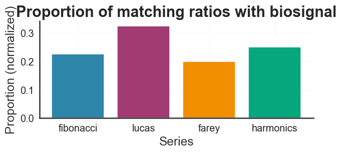
2. Which mathematical series is present?

Feed the fitted object to math_series. analyze() scores every series; the summary() table ranks them by the proportion of the EEG’s peak ratios each one reproduces.

from biotuner.math_series import math_series

ms = math_series(bt, ratios_source="peaks_ratios", maxdenom=24).analyze()
print("Best-matching series:", ms.best_series, "\n")
print(ms.summary())

Best-matching series: lucas 

      series  proportion  ...  n_target  n_series_ratios
0      lucas    0.866667  ...        15              120
1  harmonics    0.666667  ...        15               83
2  fibonacci    0.600000  ...        15               87
3      farey    0.533333  ...        15               64

[4 rows x 6 columns]

ms.plot_proportions();

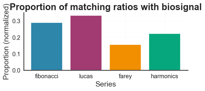
Peaks vs. extended peaks

ratios_source switches between the raw spectral peak ratios and the harmonically extended ones — they can favour different series.

ms_ext = math_series(bt, ratios_source="extended_peaks_ratios", maxdenom=24).analyze()
print("peaks    -> best:", ms.best_series)
print("extended -> best:", ms_ext.best_series)
ms_ext.plot_proportions();

peaks    -> best: lucas
extended -> best: lucas

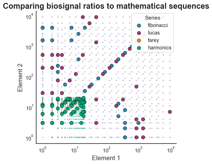
Where do the peaks sit? — the ratio-pairs scatter

Each small dot is a pair of series elements; the large dots are the pairs whose ratio matches one of the EEG’s peak ratios.

ms.plot_ratio_pairs();

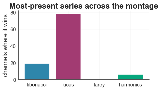
3. Across the whole montage

Running the matcher on every channel answers the population question: which series dominates this recording’s peak-ratio structure?

best_counts = {s: 0 for s in ms.series_names}
for ch in range(data.shape[0]):
    try:
        bt_ch = compute_biotuner(sf=sf, peaks_function="FOOOF", precision=0.5)
        bt_ch.peaks_extraction(data[ch], min_freq=2, max_freq=40, n_peaks=6)
        m = math_series(bt_ch, ratios_source="peaks_ratios", maxdenom=24).analyze()
        best_counts[m.best_series] += 1
    except Exception:
        continue

print("Best series per channel:", best_counts)

from biotuner.plot_config import set_biotuner_style, get_color_palette
set_biotuner_style()
plt.figure(figsize=(6, 3.2))
plt.bar(list(best_counts), list(best_counts.values()),
        color=get_color_palette("biotuner_gradient", len(best_counts)))
plt.ylabel("channels where it wins")
plt.title("Most-present series across the montage");

Best series per channel: {'fibonacci': 19, 'lucas': 78, 'farey': 0, 'harmonics': 6}

4. Derive musical structures

The matched subset of the winning series is a scale; series_mode reduces it to a consonance-selected mode.

print("Scale from best series:", [round(x, 3) for x in ms.series_scale()])
print("7-note mode (pairwise):", [round(x, 3) for x in ms.series_mode(n_steps=7, method="pairwise")])
print("Scale in cents:        ", [round(c, 1) for c in ms.scale_cents()])

Scale from best series: [1.0, 1.103, 1.103, 1.106, 1.118, 1.121, 1.131, 1.234, 1.236, 1.236, 1.236, 1.236, 1.236, 1.236, 1.236, 1.236, 1.263, 1.285, 1.286, 1.286, 1.287, 1.304, 1.306, 1.332, 1.333, 1.431, 1.455, 1.474, 1.474, 1.646, 1.958, 1.965, 1.972]
7-note mode (pairwise): [1.236, 1.236, 1.236, 1.286, 1.287, 1.474, 1.474]
Scale in cents:         [0.0, 169.2, 170.4, 173.7, 193.2, 197.8, 212.6, 364.1, 366.5, 366.8, 366.9, 366.9, 366.9, 366.9, 366.9, 367.1, 404.4, 434.0, 435.1, 436.1, 436.8, 459.9, 461.6, 496.4, 498.0, 620.3, 648.7, 671.3, 671.8, 863.3, 1163.6, 1169.8, 1175.2]

5. Creative views — where the (extended) peaks sit among the series

These are built-in math_series methods. We build a matcher on the extended-peak ratios and call each visualization. order= thins the lattice for legibility without changing the matching settings.

ms_ext = math_series(bt, ratios_source="extended_peaks_ratios", maxdenom=24).analyze()
print("best (extended):", ms_ext.best_series)
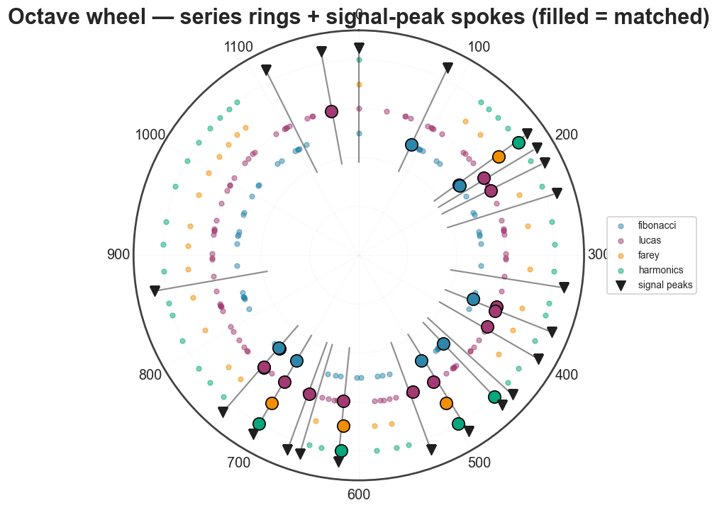
ms_ext.plot_octave_wheel(order=13);

best (extended): lucas

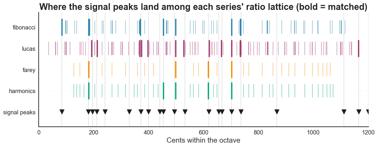
Cents ruler — the ratio lattice

Each series as a lane of ratio-ticks on a 0–1200 cents axis (bold = matched); guide lines drop from each signal peak.

ms_ext.plot_cents_ruler(order=13);

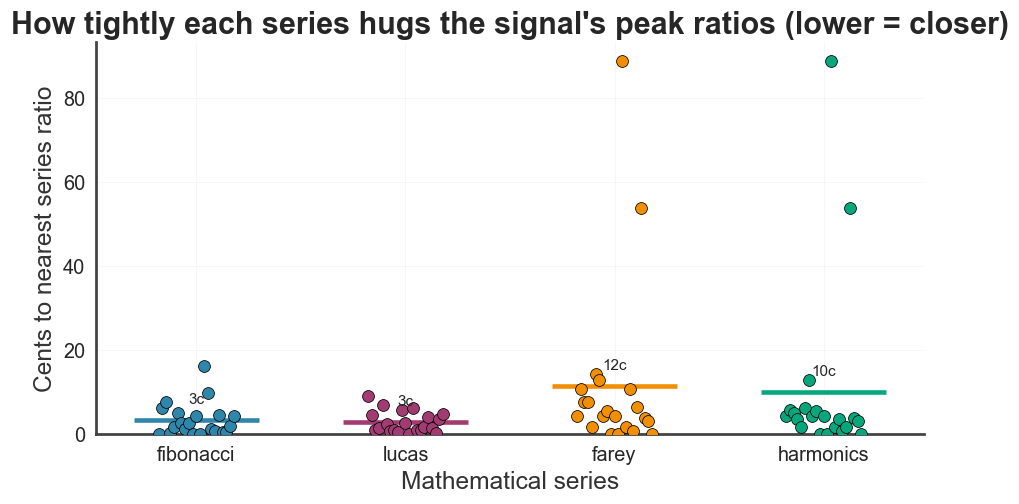
How tightly each series fits

For every extended peak, the cents distance to the nearest ratio of each series (lower = closer). A density-aware view — note Farey is dense yet does not fit tightest, so this is not just a density effect.

ms_ext.plot_fit_landscape();

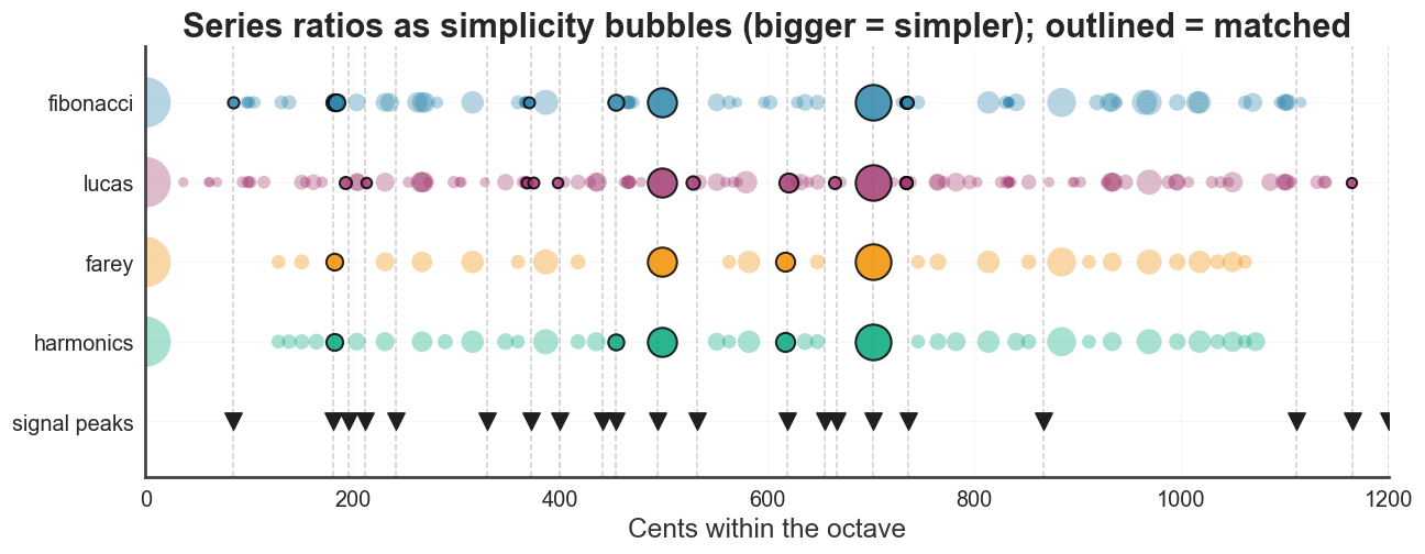
Simplicity bubbles

Each series ratio as a bubble sized by simplicity (bigger = simpler fraction). Do the signal peaks land on the simple rungs? Outlined bubbles are matched.

ms_ext.plot_simplicity_bubbles(order=13);

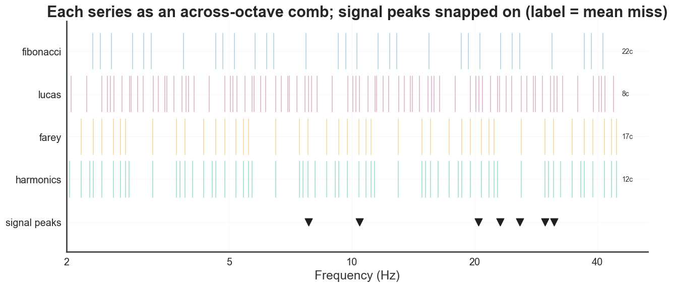
Across-octave frequency comb (the series as canvas)

Flip it around: each series, tiled across octaves and scaled to best fit the signal, becomes a frequency grid; the signal peaks (Hz) snap onto the nearest step, with each lane’s mean miss in cents.

ms_ext.plot_series_comb(order=7);

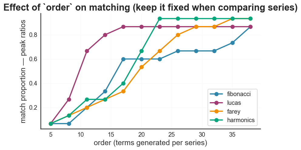
6. Effect of order on matching

order sets how many terms each series generates — more terms means a denser ratio set, which trivially matches more peaks. So the absolute proportions rise with order and then saturate. The practical lesson: keep order fixed when comparing series — only proportions computed at the same order (and maxdenom) are comparable. The ranking is usually far more stable than the absolute values.

from biotuner.plot_config import get_color_palette

orders = list(range(5, 41, 3))
series = ms.series_names
colors = dict(zip(series, get_color_palette("biotuner_gradient", len(series))))
fig, ax = plt.subplots(figsize=(8.5, 4.5))
for name in series:
    props = [math_series(bt, ratios_source="peaks_ratios", order=o, maxdenom=24)
             .analyze().series_scores[name]["proportion"] for o in orders]
    ax.plot(orders, props, "-o", color=colors[name], label=name)
ax.set_xlabel("order (terms generated per series)")
ax.set_ylabel("match proportion — peak ratios")
ax.set_title("Effect of `order` on matching (keep it fixed when comparing series)")
ax.legend();

7. Parameters to control

Parameter	Default	Controls
ratios_source	"peaks_ratios"	Which EEG ratios to analyse: raw peaks vs "extended_peaks_ratios".
maxdenom	24	Matching strictness. Ratios match if their limit_denominator(maxdenom) fractions agree. Lower (≈12–16) = lenient, higher (≈40–60) = strict. Useful range ≈16–48.
series_names	["fibonacci", "lucas", "farey", "harmonics"]	Which series to compare (also available: padovan, pell, jacobsthal, mersenne, hofstadter_q, subharmonics, triangular).
order	20	Terms generated per series (Farey order for farey); higher = denser. Keep fixed when comparing signals.
octave	2.0	Period the ratios fold into.

series_mode() adds n_steps, method ("subset" exhaustive vs "pairwise" greedy) and function (consonance metric).

Rule of thumb: the two dials you’ll actually turn are ratios_source (peaks vs extended) and maxdenom (how forgiving the match is). Keep order and maxdenom fixed across signals when comparing series — proportions are only comparable under the same settings.

All of these visualizations are methods on math_series — plot_proportions, plot_ratio_pairs, plot_octave_wheel, plot_cents_ruler, plot_fit_landscape, plot_simplicity_bubbles, and plot_series_comb — so you can call them on any biotuner object. See the biotuner.math_series API page for the full reference.